14

STRUCTURAL QUALITY ASSURANCE

Roman A. Laskowski

INTRODUCTION

The experimentally determined 3D structures of proteins and nucleic acids represent a key knowledge base from which a vast understanding of biological processes has been derived over the past half century. Individual structures have provided explanations of specific biochemical functions and mechanisms, while comparisons of structures have given insights into general principles governing these complex molecules, the interactions they make, their biological roles, and their evolutionary relationships. The 3D structures are held and looked after by the Worldwide Protein Data Bank (wwPDB) that, as of August 2007, held over 45,000 entries.

These structures form the foundation of Structural Bioinformatics; all structural analyses depend on them and would be impossible without them. Therefore, it is crucial to bear in mind two important truths about them, both of which result from the fact that they have been determined experimentally. The first is that the result of any experiment is merely a “model” that aims to give as good an explanation for the experimental data as possible. The term “structure” is commonly used, but you should realize that this should be correctly read as “model.” As such, the model may be an accurate and meaningful representation of the molecule, or it may be a poor one. The quality of the data and the care with which the experiment has been performed will determine which it is. Independently performed experiments can arrive at very similar models of the same molecule; this suggests that both are accurate representations, that they are good models.

The second important truth is that any experiment, however carefully performed, will have errors associated with it. These come in two distinct varieties: systematic errors and random errors. Systematic errors relate to the accuracy of the model—how well it corresponds to the “true” structure of the molecule in question. These often include errors of interpretation. In X-ray crystallography, for example, the molecule(s) need to be fitted to the electron density computed from the diffraction data. If the data are poor, and the quality of the electron density map is low, it can be difficult to find the correct tracing of the molecule(s) through it. A degree of subjectivity is involved and errors of mistracing and “frame-shift” errors, described later, are not uncommon, and in some cases the chain has been traced so badly as to render the final model completely wrong. In NMR spectroscopy, judgments must be made at the stage of spectral interpretation where the individual NMR signals are assigned to the atoms in the structure most likely to be responsible for them.

Random errors, on the other hand, depend on how precisely a given measurement can be made. All measurements contain errors at some degree of precision. If a model is essentially correct, the sizes of the random errors will determine how precise the model is. The distinction between accuracy and precision is an important one. It is of little use having a very precisely defined model if it is completely inaccurate.

The sizes of the systematic and random errors may limit the types of questions a given model can answer about the given biomolecule. If the model is essentially correct, but the data was of such poor quality that its level of precision is low, then it may be of use for studies of large scale properties, such as protein folds, but worthless for detailed studies requiring the atomic position to be precisely known; for example, to help understand a catalytic mechanism.

STRUCTURES AS MODELS

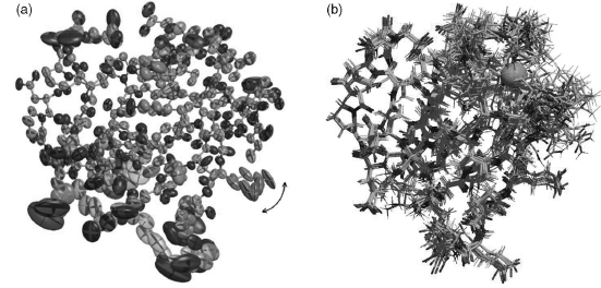
To make the point about 3D structures being merely models, it is instructive to consider the subtly different types of model obtained by the two principal experimental techniques: X-ray crystallography and NMR spectroscopy. Figure 14.1 shows the two different interpretations of the same protein given by the two methods, as explained below. The models are of the protein rubredoxin with a bound metal ion held in place by four cysteines. Both can be found in the PDB: the X-ray model (PDB code 1IRN) has a zinc as its metal ion while in the NMR model (1BFY), the metal ion is iron.

Models from X-Ray Crystallography

Figure 14.1a is a representation of the protein model as obtained by X-ray crystallography. It is not a standard depiction of a protein structure; rather, its aim is to illustrate some of the components that go into the model. The components are: the x-, y-, z-coordinates, B-factors and occupancies of all the individual atoms in the structure. These parameters, together with the theory that explains how X-rays are scattered by the electron clouds of atoms, aim to account for the observed diffraction pattern. The x-, y-, z-coordinates define the mean position of each atom while its B-factor and occupancy aim to model its apparent disorder about that mean. This disorder may be the result of variations in the atom’s position in time, due to the dynamic motions of the molecule, or variations in space, corresponding to differences in conformation from one location in the crystal to another, or both. The higher the atom’s disorder, the more “smeared out” its electron density. B-factors model this apparent smearing around the atom’s mean location; at high resolution a better fit to the “observations” can often be obtained by assuming the B-factors to be anisotropic, as represented by the ellipsoids in Figure 14.1a. Occasionally, the data can be explained better by assuming that certain atoms can be in more than one place—say, due to alternative conformations of a particular side chain (indicated by the arrows showing the two alternative positions of the glutamate side chain in Figure 14.1a). The atom’s occupancy defines how often it is found in one conformation and how often in another (for example, in Figure 14.1a the occupancy of one of the conformations of the Glu is 56% and that of the other is 44%).

Models from NMR Spectroscopy

The data obtained from NMR experiments are very different, so the models obtained differ in their nature, too. Generally, the sample of protein or nucleic acid is in solution, rather than in crystal form, which means that molecules that are difficult to crystallize, and hence impossible to solve by crystallography, can often be solved by NMR instead. The spectra measured by NMR provide a diversity of information about the molecule’s average structure in solution together with its dynamics. The most numerous, but often least precise, data are from Nuclear Overhauser Effect Spectroscop Y (NOESY) experiments where the intensities of particular signals correspond to the separations between the spatially close protons (<6A) in the structure. The spectra from Correlated Spectroscop Y (COSY)-type experiments give more precise information on the separations of protons up to three covalent bonds apart, and in some cases on the presence, or even length, of specific hydrogen bonds. Dipolar coupling experiments give information on the relative orientation of particular backbone covalent bonds (Clore and Gronenborn, 1998).

The proton separations obtained from the experimental data are converted into distance and angular restraints that are used to generate models of the structure that are consistent with these restraints. Various techniques are used to obtain these models; the most commonly used are molecular dynamics based simulated annealing procedures similar to those used in X-ray structure refinement. The end result is not a single model, but rather an ensemble of models that are all consistent with the given restraints, as illustrated in Figure 14.1b.

The reasons for generating an ensemble of structures from NMR data are twofold. Firstly, the NMR data are relatively less precise and less numerous than experimental restraints from X-rays, so a diversity of structures are consistent with them. Secondly, the molecules may genuinely possess heterogeneity in solution. In fact, it has even been suggested that low-resolution X-ray models would benefit from being generated as ensembles, much like their NMR counterparts, to better represent the experimental data (DePristo, de Bakker, and Blundell, 2004).

For general use, an ensemble of models is rather more difficult to handle than a single model. Ensembles deposited in the PDB can typically comprise 20 models, with the largest ensemble in the PDB, as of August 2007, having 184 models (PDB code 2HYN; Potluri et al., 2006). One of the models may be designated the“representative” of the whole ensemble, or, alternatively, a separate averaged model may be computed from all the ensemble members. This “average structure” has tobe energy minimized to counteract the unphysicalbond lengths and angles that the averaging process introduces. Such a structure tends to have a separate PDB identifier from that of the ensemble—so the same structure, or rather the outcome of the same experiment, appears as two separate entries in the PDB. This is clearly potentially confusing and the use of separate files is now discouraged. The representative member of an ensemble is usually taken to be the structure that differs least from all other structures in the ensemble. An algorithmic Web-based tool called OLDERADO (Kelley, Gardner, and Sutcliffe, 1996) allows to select such a representative from an ensemble (http://www.ebi.ac.uk/msd-srv/olderado), but no single algorithm is universally agreed upon.

Models from Electron Microscopy (EM)

X-ray and NMR models are by far the most common of the experimentally determined models of macromolecular structures. However, there are a small number of models in the PDB (153 models as of August 2007) that have been derived from electron microscopy (EM) experiments, and these require special caution. The experimental data underlying these models is of especially low resolution, typically in the range of 6-15Å —well below the limits where individual side chains, let alone atoms, can be discerned—and the structures tend to be of large multiprotein and/or RNA complexes. Yet the models in the PDB entries do contain atomic coordinates; usually, just the C^α backbone atoms, but in some cases all main chain and side chain atoms! The latter are derived by fitting the coordinates of one or more crystal structures, solved at higher resolution, into the EM maps. The resultant coordinates of the final model are, at best, an approximation of the atomic positions of the various components making up the sample and will not have been subjected to any rigorous positional or geometric refinement procedures. Consequently, they should not be relied on to any great extent.

Other Experimentally Determined Models

The PDB also contains models solved by powder, fiber, electron and neutron diffraction studies as well as electron tomography, infrared spectroscopy and solution scattering. Each method has its strengths, weaknesses, and peculiarities, so structures solved by these methods need to be carefully assessed on a case-specific basis, with reference to the literature describing them.

Theoretical Models

Particular skepticism should be reserved for models that are not directly based on any experimental measurement. These are the so-called “theoretical models” and are obtained either by homology modeling or “threading” techniques. Homology models rely on the fact that proteins sharing high-sequence identity tend to have very similar overall 3D structures; proteins sharing a sequence identity greater than around 35% will have essentially the same fold. This makes it possible to generate a “homology model” of the 3D structure of a given protein based on the 3D model of a closely related protein. The modeling can be automated and there are several servers that generate models from user-submitted sequences, the best known being SWISS-MODEL (Schwede et al., 2003). Even where the model is a good one, that is, obtained from a very similar protein, one needs to be cautious about taking the model’s atomic positions at face value as they do not represent positions based on any experimental data. In fact, it is likely that any experimental errors in the template model will not only be propagated into the homology model but even exacerbated in the process.

The PDB, which used to treat theoretical models much like experimentally derived ones, has, since July 2002, kept them apart in a separate ftp site: ftp://ftp.wwpdb.org/pub/pdb/data/structures/models/current. New models are no longer accepted (Berman et al., 2006). As of August 2007, there were 1358 theoretical models on the models site.

The least reliable models of all are predicted models such as those generated by ab initio and fold recognition or “threading” methods. These methods can be described as straw-clutching measures of last resort, employed when a given protein sequence has no relatives in the PDB and so is not amenable even to homology modeling. Occasionally, these methods approximate the right answer—usually for small, single-domain proteins where they may produce topologically near correct models (Moult, 2005)—but generally, they are wildly wrong. So, it is safe to assume that the level of error in any such model will be high.

AIMS

The primary take-home message of this chapter is that not all structural models, whether in the PDB or not, are equally reliable and each should be critically assessed before being used for one’s own work. It may seem slightly churlish to reject any structure given the amount of time, care, and hard work, the experimentalists or modelers may have put into creating it; but ifyou put unsound data into your analysis, you will get unsound conclusions out ofit. Some models will be unreliable simply because the experimental data from which they were derived were of poor (or nonexistent) quality, while others may be unreliable as a result of human error. Whatever the reason, it is important to weed out any uncertain models as early as possible.

This chapter aims to explain the problems of relying on 3D models uncritically and provides some rules of thumb for filtering out the defective ones: what are the symptoms to look for, how to detect them, and at what point should you reject a model?

ERROR ESTIMATION AND PRECISION

All scientific measurements contain errors. No measurement can be made infinitely precisely; so, at some point, say after so many decimal places, the value quoted becomes unreliable. Scientists acknowledge this by estimating and quoting standard uncertainties on their results. For example, the latest value for Boltzmann’s constant is 1.3806503(24) x 10~²³ J/K, where the two digits in brackets represent the standard uncertainty (s.u.) in the last two digits quoted for the constant.

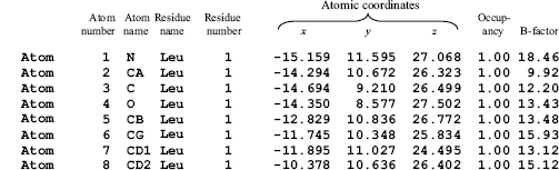
Compare this with the situation we have in relation to the 3D structures of biological macromolecules. Figure 14.2 shows a typical extract from the atom details section of a PDB file. It relates to a single amino acid residue (a leucine) and shows the information deposited about each atom in the protein’s structure.

Looking at only the columns representing the x-, y-, z-coordinates you’ll notice that each value is quoted to three decimal places. This suggests a precision of about 1 in 10⁵ in the given example. Similarly, the B-factors (in the final column) are each quoted to two decimal places. Is it possible that the atomic positions and B-factors were really so precisely defined? What are the error bounds on these values? Are the values accurate to the first place of decimals? The second? The third?

In fact, with the exception of a very few PDB structures, no error bounds are given. As of August 2007, there were 10 such exceptions, out of over 45,000 structures, the largest being a protein chain of 313 amino acid residues and four bound ligands (human aldose reductase, PDB code 2I17). All the 10 had been solved at atomic resolution (ranging from 0.89 to 1.3 A) and refined by the full-matrix least squares method that will be discussed later.

Thus, in the overwhelming majority of cases one cannot tell how precisely defined the values are. Why is this so? What kind of scientific measurement is this? And how are we to judge how much reliance should be placed on the data given?

ERROR ESTIMATES IN X-RAY CRYSTALLOGRAPHY

Estimation of Standard Uncertainties

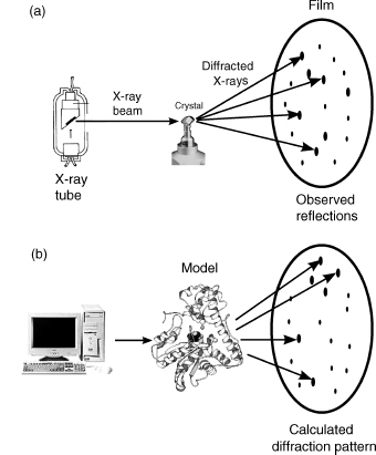
In X-ray crystallography, it is actually possible, in theory, to calculate the standard uncertainties of the atomic coordinates and B-factors. In fact, it is routinely done for the X-ray crystal structures of small molecules such as those deposited in the Cambridge Structural Database (CSD) (Allen et al., 1979). The calculations of the s.u.s are performed during the refinement stage of the structure determination. As you learnt in Chapter 4, refinement involves modifying the initial model to improve the match between the experimentally determined structure factors—as obtained from the observed X-ray diffraction pattern—and the calculated structure factors—as obtained from applying scattering theory to the current model of the structure. Figure 14.3 illustrates this principle.

In practice, refinement is usually a long drawn-out procedure requiring many cycles of computation interspersed here and there with manual adjustments of the model using molecular graphics programs to nudge the refinement process out of any local minimum that it may have become trapped in. Furthermore, because in protein crystallography, the data-to-parameter ratio is poor (the data being the reflections observed in the diffraction pattern and the parameters being those defining the model of the protein structure: the atomic x-, y-, z-coordinates, B-factors, and occupancies) the data needs to be supplemented by additional information. This extra information is applied by way of geometrical restraints. These are “target” values for geometrical properties such as bond lengths and bond angles and are typically obtained from crystallographic studies of small molecules. The refinement process aims to prevent the bond lengths and angles in the model drifting too far from these target values. This is achieved by applying additional terms to the function being minimized of the form:

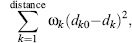
where d_k and d_k0 are the actual and target distance, and Wk is the weight applied to each restraint.

If the structure is refined using full-matrix least-squares refinement, a by-product of this method is that the s.u.s of the refined parameters, such as the atomic coordinates and B-factors, can be obtained. However, their calculation involves inverting a matrix the size of which depends on the number of parameters being refined. The larger the structure, the more atomic coordinates and B-factors, the larger the matrix. As matrix inversion is an order n³ process, it has tended to be unfeasible for molecules of the size of proteins and nucleic acids; these have several thousand parameters and consequently a matrix whose elements number several millions or tens of millions. This is why s.u.s have been routinely published for small-molecule crystal structures, but not for structures of biological macromolecules. It is purely a matter of size.

However, as faster workstations with larger memories have become available, the situation has started to change, and calculation of atomic errors has become more practicable (Tickle et al., 1998). Indeed, s.u.s are now frequently calculated for small proteins using SHELX (Sheldrick and Schneider, 1997), the refinement package originally developed for small molecules, but sadly, the s.u. data are still not commonly deposited in the PDB file. So this makes us none-the-wiser about the precision with which any given atom’s location has been determined.

So what is to be done? What other information is there on the reliability of an X-ray crystal structure? What should one look for?

First of all, one can get an idea of the global quality of the structure from certain parameters that are commonly cited in the literature and quoted in the header records of the PDB file itself, as described next.

Global Parameters for X-Ray Structures

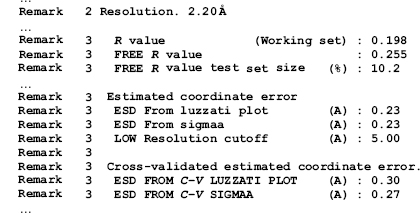
Figure 14.4 shows an extract from the header records of a PDB file showing some of the commonly cited global parameters.

Resolution. The resolution at which a structure is determined provides a measure of the amount of detail that can be discerned in the computed electron density map. The reflections at larger scattering angles, θ, in the diffraction pattern correspond to higher resolution information coming as they do from crystal planes with a smaller interplanar spacing. The high-angle reflections tend to be of a lower intensity and more difficult to measure and the greater the disorder in the crystal, the more of these high-angle reflections will be lost. Resolution relates to how many of these high-angle reflections can be observed, although the value actually quoted can vary from crystallographer to crystallographer, as there is no clear definition of how it should be calculated. The higher resolution shells will tend to be less complete and some crystallographers will quote the highest resolution shell giving a 100% complete data set, whereas others may simply cite the resolution corresponding to the highest angle of scatter observed.

The higher the resolution, the greater the level of detail, and hence the greater the accuracy of the final model. The resolution attainable for a given crystal depends on how well ordered the crystal is, that is, how close the unit cells throughout the crystal are to being identical copies of one another. A simple rule of thumb is that the larger the molecule, the lower will be the resolution of the data collected.

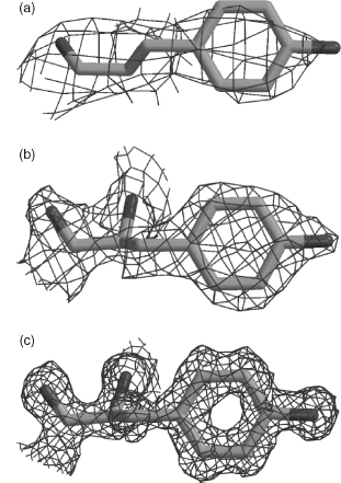
Figure 14.5 shows an example of how the electron density for a single side chain improves, as resolution increases. In general, side chains are difficult to make out at very low resolution (4 Å or lower), and the best that can be obtained is the overall shape of the molecule and the general locations of the regions of regular secondary structure. Models at such low resolution are clearly of no use for investigating side chain conformations or interactions! At 3 Å resolution, the path of a protein’s chain can be traced through the density and at 2 Å, the side chains can be confidently fitted.

The mostprecise structures are the atomic resolution ones (from around 1.2 Å resolution up to around 0.9 Å). Here the electron density is so clear that many of the hydrogen atoms become visible, and alternative occupancies become more easily distinguishable. These structures require fewer geometrical constraints during refinement and hence give a better indication of the true geometry of protein structures.

The resolution of X-ray structures in the PDB varies from atomic resolutions structures to very low-resolution structures at around 4.0 Å, with a definite peak at around 2.0 Å. Structures solved at resolutions below 4 Å tend to be solved by electron microscopy. The lowest quoted resolution, as at August 2007, was 70.0 Å for a whole series of structural models of skeletal muscle crossbridges in insect flight muscle, solved by electron tomography; for example, PDB entry 1M8Q (Chen et al., 2002).

Resolution is probably the clearest measure of the likely quality of the given model. However, bear in mind that, because there is no single, consistent definition of resolution its value can be overstated (Weissig and Bourne, 1999). What is more, in X-ray crystallography poor resolution data can sometimes result in models of quite respectable quality if the crystals exhibit a high degree of noncrystallographic symmetry. By averaging the data at symmetry related positions one can build models that would otherwise be impossible. This is the trick that allows very large complexes such as the protein coats of viruses to be solved crystallographically despite apparently poor data.

R-Factor. The R-factor is a measure of the difference between the structure factors calculated from the model and those obtained from the experimental data. In essence, it is a measure of the differences in the observed and computed diffraction patterns schematically illustrated in Figure 14.3. Higher values correspond to poorer agreement with the data, while lower values correspond to better agreement. Typically, for protein and nucleic acid structures, values quoted for the R-factor tend to be around 0.20 (or equivalently, 20%). Values in the range 0.40-0.60 can be obtained from a totally random structure, so structures with such values are unreliable and probably would never be published. Indeed, 0.20 seems to be something of a magical figure and many structures are deemed finished once the refinement process has taken the R-factor to this mystical value.

As a reliability measure, however, the R-factor is in itself somewhat unreliable. It is quite easily susceptible to manipulation, either deliberate or unwary, during the refinement process, and so models with major errors can still have reasonable-looking R-factors. For example, one of the early incorrect structures, cited by Branden and Jones (1990), was that of ferredoxin I, an electron transport protein. The fully refined structure was deposited in 1981 as PDB code 2FD1, with a quoted resolution of 2.0 Å and an R-factor of 0.262. Due to the incorrect assignment of the crystal space group during the analysis of the X-ray diffraction data, this structure turned out to be completely wrong. The replacement structure, reanalyzed by the original authors and having the correct fold, was deposited as PDB entry 3DF1 in 1988. Its resolution was given as 2.7 Å and its R-factor as 0.35. On the face of it, therefore, mere comparison of the resolution and R-factor parameters would lead one to believe the first of the two structures to be the more reliable! The reason why an R-factor as low as 0.262 was achieved for a totally incorrect structure was that the coordinates included 344 water molecules, many extending far out from the protein molecule itself. This is a large number of waters for a protein containing only 107 residues. A well-known rule of thumb suggests that a reasonable number of waters in a given structure is roughly one water molecule for each protein residue, and waters should only be added to the structure if they make plausible hydrogen bonds. This “one water per residue” rule has been shown to be true for structures solved at around 2 Aresolution, although at higher resolution more waters can be detected; at 1.0 Aresolution one can reasonably expect to detect 1.6-1.7 waters per residue (Carugo and Bordo, 1999).

Incidentally, the 3DF1 model of ferredoxin has itself been twice superseded: first by entry 4df1 in mid-1988 and then by entry 5DF1 in 1993. The last of these had a quoted resolution of 1.9 A and R-factor of 0.215.

The ferredoxin case is one of overfitting, that is, having too many parameters for the available experimental data. In the original 2FD1 model, the discrepancy between the observed and computed diffraction patterns was literally washed out by the addition of so many water molecules. One can always fit a model, however wrong, to the experimental data and obtain a reasonable R-factor if there is an excess of parameters over observations.

R_free. A more reliable reliability factor is Briinger’s free R-factor, or R_free (Bruanger, 1992). This is less susceptible than the standard R-factor to manipulation during refinement. It is calculated in the same way, but using only a small fraction of the experimental data, typically 5-10%. Crucially, this fraction, known as the test set, is excluded from the structure refinement procedure that uses the remaining 90-95% of the data, or working set. Thus, unless there are correlations between the data in the test and working sets, the R_free provides an independent measure of the fit of the model to the data and cannot be biased by the refinement process.

The value of R_free will tend to be larger than the R-factor, although it is not clear what a good value might be. Brunger has suggested that any value above 0.40 should be treated with caution (Briunger, 1997). There were 51 structures in the PDB, as of August 2007, in this category. Not surprisingly, most are fairly low-resolution structures, solved at 3.0 Aor lower, but a few, rather worryingly, are not.

Average Positional Error. Even though atomic coordinate s.u.s are not commonly given, it is quite usual for an estimate of the average positional error of a structure’s coordinates to be cited. There are two principal methods for estimating the average positional errors: the Luzzati plot (Luzzati, 1952) and the σ_A plot (Read, 1986).

The Luzzati plot is obtained by partitioning the reflections from the diffraction pattern into bins according to their value of sin θ, where θ is the reflection’s scattering angle, and then calculating the R-factor for each bin. The value calculated for each bin is plotted as a function of sin θ/λ, where λ is the wavelength of the radiation used. The resulting plot is compared against the theoretical curves of Luzzati (1952) to obtain an estimate of the average positional error. One problem with this method is that the actual curves do not usually resemble the theoretical ones well at all, and so the error estimate is somewhat crude and often merely provides an upper limit on the error. Better results are obtained if the R_free is used instead of the traditional R-factor.

The σ_A plot provides a better estimate. It involves plotting ln σ_A against (sin θ/λ)², where σ_A is a complicated function that has to be estimated for each (sin θ/λ)² bin, as described in Read (1986). The resultant plot should give a straight line the slope of which provides an estimate of the average positional error.

Most refinement programs compute both the Luzzati and Read error estimates, so these values are commonly cited in the PDB file. You will find them in the file’s header records under the now unfashionable term “estimated standard deviation” (ESD) (see Figure 14.4).

Bear in mind that an average s.u. is exactly what it says: an average over the whole structure. The s.u.s of the atoms in the core of the molecule, which tends to be more ordered, will be lower than the average, while those of the atoms in the more mobile and less well-determined surface—and often more biologically interesting—regions will be higher than the average.

Atomic B-Factors. A more direct, albeit merely qualitative, way of determining the precision of a given atom’s coordinates is to look at its associated B-factor. B-factors are closely related to the positional errors of the atoms, although the relationship is not a simple one that can be easily formulated (Tickle et al., 1998). It is safe to say, however, that atoms in a structure with the largest B-values will also be those having the largest positional uncertainty. So if high levels of precision are required in your analysis, leave out the atoms having the highest B-factors. As arule of thumb, atoms with B-values in excess of 40.0 are often excluded as being too unreliable. Similarly, if atoms in your region of interest, such as an active site, are all cursed with high B-factors then your region of interest is not well determined and you will either need to be careful about the conclusions you draw from it, or else seek out a different structural model of the same protein where the region is better defined.

Other Parameters. The above parameters are those that are commonly given in the header records of the PDB entry but are by no means the only information that can be used for assessing the usefulness of a given structural model. Other checks, such as on the geometry of the model or its agreement with the experimental data can be made by running the appropriate software or accessing the appropriate Web server, as will be discussed later.

Rules of Thumb for Selecting X-Ray Crystal Structures

Many analyses in Structural Bioinformatics require the selection of a dataset of 3D structures on which analysis can be performed. A commonly used rule of thumb for selecting reliable structures for such analyses, where reasonably accurate models are required, is to choose those models that have a quoted resolution of 2.0 A or better, and an R-factor of 0.20 or lower. These criteria will give structures that are likely to be reasonably reliable down to the conformations of the side chains and local atom-atom interactions. One example that uses such a dataset is the Atlas of Protein Side Chain Interactions (http://www.ebi.ac.uk/thornton-srv/databases/sidechains) that depicts how amino acid side chains pack against one another within the known protein structures.

Of course, the selection criteria depend on the type of analysis required. For some analyses, only atomic resolution structures (i.e., 1.2 A or better) will do, as in the accurate derivation of geometrical properties of proteins; for example, side chain torsional con-formers and their standard deviations (EU 3D Validation Network, 1998), or fine details of the peptide geometry in proteins that can reveal subtle information about their local electronic features (Esposito et al., 2000). For other types of analysis, structures solved down to 3 A may be good enough, as in any comparison of protein folds. One interesting example is that of the lactose operon repressor. Three structures of this protein were solved to 4.8 Aresolution, giving accurate position for only the protein’s C^α atoms (Lewis et al., 1996). However, because the three structures were of the protein on its own, of the protein complexed with its inducer, and of the protein complexed with DNA, the global differences between the three structures showed how the protein’s conformation changed between its induced and repressed states. Thus, even these very low-resolution structures were able to help explain how this particular protein achieves its biological function (Lewis et al., 1996).

Often the above rule of thumb (resolution ≤2.0 Å, and R-factor ≤0.20) is supplemented by a check on the year when the structure was determined. Structures are more likely to be less accurate, the older they are simply because experimental techniques have improved markedly since the early pioneering days of the 1960s and 1970s (Weissig and Bourne, 1999; Kleywegt and Jones, 2002). Indeed, many of the early structures have been replaced by more recent and accurate determinations.

ERROR ESTIMATES IN NMR SPECTROSCOPY

The theory of NMR spectroscopy does not provide a means of obtaining s.u.s for atomic coordinates directly from the experimental data, so estimates of a given structure’s accuracy and precision have to be obtained by more indirect means.

Global Parameters for NMR Structures

As mentioned above, a number of models can be derived that are compatible with the NMR experimental data. It is difficult to distinguish whether this multiplicity of models reflects real motion within the molecules or simply results from insufficient experimentally derived restraints. (Compare how the most poorly defined regions of the X-ray model of rubredoxin in Figure 14.1a do not necessarily correspond to the most poorly defined regions of the NMR model in Figure 14.1b, although remembering that one structure was in crystal form, and the other in solution.) Generally, the agreement of NMR models with the NMR data is measured by the agreement between the distance and angular restraints applied during the refinement of the models and the corresponding distances and angles in the final models. Large numbers of severe violations indicate a serious problem of data interpretation and model building.

However, the errors associated with the original experimental data are sufficiently large that it is almost always possible to generate models that do not violate the restraints, or do so only slightly. Consequently, it is not possible to distinguish a merely adequate model from an excellent one by looking for restraint violations alone.

Traditionally, the “quality” of a structure solved by NMR has been measured by the root-mean-squared deviation (RMSD) across the ensemble of solutions. Regions with high RMSD values are those that are less well defined by the data. In principle, such RMSD measures could provide a good indicator of uncertainty in the atomic coordinates; however, the values obtained are rather dependent on the procedure used to generate and select models for deposition. An experimentalist choosing the “best” few structures for deposition from a much larger draft ensemble can obtain very misleading statistics for the PDB entry. For example, the “best” few structures may, in effect, be the same solution with minor variations, so the RMSD values will be small. Structures further down the original list may provide alternative solutions, which are slightly less consistent with the data, but which are radically different.

The number of experimentally derived restraints per residue gives another measure of quality. This provides an indication of how effectively the NMR data define the structure in a manner analogous to the resolution of X-ray structures. Indeed, the number of restraints per residue correlates with the stereochemical quality of the structures to an extent, but some restraints may be completely redundant and no consistent method of counting is used by depositors. A better guide is the completeness of NOEs (Doreleijers et al., 1999) that compares the numbers of NOEs that one would expect to get, given the final model, against the number that were actually observed. The completeness gives a slightly better correlation with stereochemical parameters. However, the calculation of expected NOEs is complicated by the fact that it is made from a static model, so some expected NOEs may not in fact be detectable due to the internal dynamics of the molecule in question.

None of the above measures gives a true indication of the accuracy of the models—that is, how well they represent the true structure—and few of them are reported in the PDB file.

In recent years, NMR equivalents of the crystallographic R-factor have been introduced. One method involves the use of dipolar couplings. These provide long-range structural restraints that are independent of other NMR observables such as the NOEs, chemical shifts, and couplings constants that result from close spatial proximity of atoms. Because the expected dipolar couplings can be computed for a given model, they provide a means of comparing the observed with the expected, and obtaining an R-factor that is a measure of the difference between the two (Clore and Garrett, 1999). What is more, it is also possible to obtain a cross-validated R-factor, equivalent to the crystallographic R_free, wherein a subset of dipolar couplings are removed prior to the start of structure refinement and used only for computing the R-factor. This gives an unbiased measure of the quality of the fit to the experimental data. However, in the case of NMR, one cannot use a single test set of data; one has to perform a complete cross-validation. The reason for this is that, whereas in crystallography each reflection contains information about the whole molecule, in NMR each dipolar coupling does not. So a complete cross-validation is required, which means that a number of calculations have to be performed, each using a different selection of test and working data sets; the test set, which usually comprises 10% of the whole data set, being selected at random each time.

Another technique for calculating an NMR R-factor uses the NOEs and involves back calculation of the NMR intensities from the models obtained and comparison with those observed in the experiment. This technique is implemented in the program RFAC (Gronwald et al., 2000) that calculates not only an overall R-factor for the entire structure, but also local R-factors, including residue-by-residue R-factors and individual R-factors for different groups of NOEs (e.g., medium range NOEs, long range NOEs, inter-residue NOEs, etc.).

An additional back-calculation method for checking structure quality is to calculate the expected frequencies (positions) of spectral peaks from the structure and compare them with those observed. This comparison has the advantage that the frequencies are not usually a target of the structure refinement procedure (Williamson, Kikuchi, and Asakura, 1995).

However, once again, the measures described here are not generally included in the deposited PDB files and so have to be laboriously obtained from the relevant literature reference.

Rules of Thumb for Selecting NMR Structures

Historically, the rule of thumb for selecting NMR structures for inclusion in structural analyses has been the simple one of excluding them altogether! This early prejudice stems from the fact that they were viewed as being of generally lower quality than X-ray structures as a number of studies have been keen to point out (see Spronk et al., 2004, and references therein). There has never been an easy way of distinguishing the good from the bad NMR models using a simple rule of thumb as in the case of X-ray structures. However, NMR structures provide much valuable information about protein and DNA structures not available from X-ray studies. For example, just under 15% of PDB structures come from NMR experiments (as at August 2007), although, as mentioned previously, this includes a lot of double counting with many structures being deposited as two separate PDB entries: one for the whole ensemble and the other for an energy minimized average structure. So in terms of models derived from separate NMR experiments, this percentage is far lower. However, when one selects data sets of nonhomologous sequences in the PDB at the 30% sequence identity level, one finds that just over 16% are NMR structures. So to exclude all NMR models involves discarding many unique and important proteins that perhaps can only ever be solved by NMR.

Because there is no standard information provided in the header information of NMR PDB files relating to either the quality of the experimental data or the resultant models, one has to either read and interpret the original paper describing the structure or, more practically, rely on measures of the stereochemical quality of the structure, as will be described later.

There are two very useful Web sites that provide “improved” versions of several hundred old NMR models. The improved models have been generated by re-refining the original experimental data using more up-to-date force fields and refinement protocols. The first is DRESS, a Database of Refined Solution NMR Structures (Nabuurs et al., 2004), which contains 100 re-refined NMR models (http://www.cmbi.kun.nl/dress) and the second, more recent, database is RECOORD (Nederveen et al., 2005) that contains 545 models (http://www.ebi.ac.uk/msd/NMR/recoord). Along with giving the new coordinates, the databases provide indicators of how the newer models are an improvement over the old in terms of stereochemical quality measures. So, if the structure you need is an early NMR model, it is worth checking whether it is included in either of these two databases.

ERRORS IN DEPOSITED STRUCTURES

Serious Errors

At the end of 2006, a letter to the journal “Science” caused something of a stir in the structural biology community. The authors wrote to say that they were withdrawing three of their Science papers, and five corresponding PDB entries, due to serious errors in their models (Chang et al., 2006). The errors were the result of a trivial mistake made during initial processing of the X-ray data. As a consequence, the final models had serious errors in their handedness and topology as was revealed when another group solved a similar structure.

Such a high profile retraction is fairly rare but the concern about serious errors in structural models has been around for a long time (Brändén and Jones, 1990) and there have been a number of serious errors in both X-ray and NMR structures documented in the literature (Kleywegt, 2000). As in the example above, many of the erroneous models have been retracted by their original authors, or replaced by improved versions. It is common for structures to be re-refined, or solved with better data, and the models in the PDB replaced by the improved versions. So it is instructive to bear in mind that, at any time, there are likely to be models in the PDB that are in need of replacement!

The old models do not all disappear. There is a growing graveyard of “obsolete” structures—some very much incorrect, others merely slightly mistaken—available from the wwPDB (ftp://ftp.wwpdb.org/pub/pdb/data/structures/obsolete).

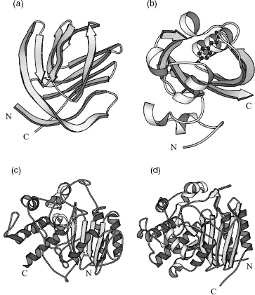
Of all the errors, the most serious are those where the model is, essentially, completely wrong such as when the trace of the protein chain follows the wrong path through the electron density resulting in a completely incorrect fold. One example, that of ferredoxin I, has already been mentioned in the discussion of the crystallographic R-factor above. Another example is depicted in Figures 14.6a and b that show an incorrect and correct model of photoactive yellow protein. There is practically no similarity between the two.

The next most serious errors are where all, or most, of the secondary structural elements have been correctly traced, but the chain connectivity between them is wrong. An example is given in Figures 14.6c and d. Here the erroneous model has most of the correct secondary structure elements, and has them arranged in the correct architecture, but the protein sequence has been incorrectly traced through them (in one case going the wrong way down a p-strand). Consequently, most of the protein’s residues have ended up in the wrong place in the 3D structure. Errors such as this arise because the loop regions that connect the secondary structure elements tend to be more flexible, and more disordered, so their electron density tends to be more poorly defined and difficult to interpret correctly. In the case shown in Figure 14.6c, the interpretation of the electron density was made especially difficult by the simple fact that the primary sequence of the protein was unknown at the time. Thus, the sequence of the protein had to be inferred from the blobs of electron density as the chain was being fitted into it; usually, the sequence is a crucial guide to the tracing of the protein chain. Needless to say, it was subsequently found that the inferred primary sequence was just as much in error as the 3D structure.

Less serious are frame shift errors, although they can often result in a significant part of the model being incorrect. These errors occur where a residue is fitted into the electron density that belongs to the next residue. The frame shift persists until a compensating error is made when two residues are fitted into the density belonging to a single residue (Jones and Kjeldgaard, 1997). These mistakes often occur in loop regions, and almost exclusively at very low resolution (3 Å or lower). Frame shift errors were recently investigated in a data set of 842 protein chains belonging to the oligosaccharide binding (OB)-fold (Venclovas, Ginalski, and Kang, 2004). Of the 842 chains, 12 (1.4%) were found to have frame shift errors. The 12 chains were contained in five separate PDB entries (some of which were multimers) deposited between 1983 and 2000 and ranging in resolution from 2.2 to 3.2 Å.The authors of the study concluded that around 1% of all protein sequences in the PDB could contain such errors.

The least serious model-building errors involve the fitting of incorrect main chain or side chain conformations into the density. Of course, even such errors, depending on where they occur, can have an effect on the biological interpretation of what the structure does and how it does it.

Typical Errors

Typically, the majority of the models deposited in the PDB will be essentially correct. The remaining errors will be the random errors associated with any experimental measurement. As mentioned above, for X-ray structures, the average s.u.s—estimated on the basis of the Luzzati and σ_A plots—can provide an idea of the magnitude of these errors. The values range from around 0.01 to 1.27 Å. Note that the latter value approaches the length of some covalent bonds! The median of the quoted s.u.s corresponds to estimated average coordinate errors of around 0.28 A. It has to be remembered that these values are estimates, and are applied as an average over the whole model.

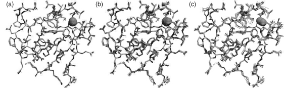
Figure 14.7 gives a feel of some typical uncertainties in atomic positions, showing positional uncertainties of 0.2, 0.3, and 0.39 Å.

A surprising result from a recent study was that some types of errors that are relatively easy to detect and fix were still turning up in newly released PDB entries (Badger and Hendle, 2002). The authors found that, in the PDB entries they looked at (all released on a single day) 3.6% of the amino acids contained an error of some kind, with the worst model having errors in 10.6% of its amino acids. The most common errors were His/Asn/Gln side chain flips. These side chains are symmetrical in terms of shape and so will fit their electron density equally well when rotated by 180°. However, their chemical properties are not symmetrical and, in general, one orientation will result in a better hydrogen-bonding network than the other. This can be critical when the side chain in question is part of a catalytic or binding site and all such errors should really have been fixed prior to the deposition of the models in the PDB.

STEREOCHEMICAL PARAMETERS

Given that all structural models contain some degree of error, what else, other than the global parameters described above, can help assess the quality of each one? On every powerful class of checks are those that examine a model’s geometry, stereochemistry and other structural properties. These checks compare a given protein or nucleic acid structure against what is already known about these molecules. The “knowledge” comes from high-resolution structures of small molecules plus systematic analyses of the existing protein and nucleic acid structures in the PDB. The latter analyses rely on the vast body of structures solved to date providing a knowledge base of what is “normal” for these biomolecules.

The advantage of such tests of “normality” is that they do not require access to the original experimental data. Although it is possible to obtain the experimental data for many PDB entries—structure factors in the case of X-ray structures, and distance restraints for NMR ones—this is still the minority of entries, and deposition of these data is still at the discretion of the depositors. Furthermore, to make use of the data requires appropriate software packages and expert know-how. The stereochemical tests, on the contrary, require no experimental data and are easy to run and understand. So, in fact, any 3D structure, whether experimentally determined, or the result of homology modeling, molecular dynamics, threading or blind guesswork can be checked. The software for checking structures is freely available and there are now many Web servers that provide these checks for you, as will be mentioned later.

Before describing the checks, one crucial point needs to be stressed at the start. The majority of the checks compare a given structure’s properties against what is the “norm.” Yet this norm has been derived from existing structures and could be the result of biases introduced by different refinement practices. Furthermore, outliers, such as an excessively long bond length, or an unusual torsion angle, should not be construed as errors. They may be genuine, for example, as a result of strain in the conformation, say, at the active site. The only way of verifying whether oddities are errors or merely oddities is by referring back to the original experimental data. Indeed, the experimenters who solved the structure may already have done this, found the apparent oddity to be correct and commented to that effect in the literature.

Having said that, if a single structure exhibits a large number of outliers and oddities, then it probably does have problems and perhaps should be excluded from any analyses.

Proteins

The Ramachandran Plot. For proteins, the best known, and most powerful, check of stereochemical quality is the Ramachandran plot (Ramachandran, Ramakrishnan, and Sasisekharan, 1963). This is a plot of the ψ main chain torsion angle versus the main chain torsion angle (see Chapter 2) for every amino acid residue in the protein (except the two terminal residues because the N-terminal residue has no and the C-terminus has no ψ). In the resulting -ψ scatterplot, the points tend to be excluded from certain “disallowed” regions and have a tendency to cluster in certain favorable regions (Figure 14.8). The disallowed regions are where steric hindrance between side chain atoms makes certain -ψ combinations difficult or even impossible to achieve. Glycine, which has no side chain to speak of, has a much greater freedom of movement in terms of its -ψ combinations, although it still has regions from which it is excluded (Figure 14.8b). Conversely, proline, which has two covalent connections to the backbone, is more restricted than other amino acids and its accessible regions of the -ψ plot are confined to a narrow range of values (Figure 14.8c).

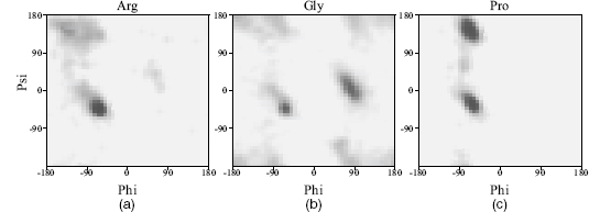
The favorable regions on the plot correspond to the regular secondary structures: right-handed helices, extended conformation (as found in β-strands), and left-handed helices. These are the dark regions in Figure 14.9 labeled A, B, and L, respectively. Even residues in loops tend to lie within these favored regions. Figure 14.9a shows a typical Ramachandran plot with the residues showing a tight clustering in the most favored regions with few or none in the disallowed regions. The favorable and disallowed regions are determined from analyses of existing structures in the PDB (Morris et al., 1992; Kleywegt and Jones, 1996).

Figure 14.9b shows a somewhat pathological Ramachandran plot. It comes from a structure that shall remain nameless. Here, the majority of the residues lie in the disallowed regions and it can be confidently concluded that the model has serious problems.

One caveat concerns proteins containing D-amino acids rather than the more common L-amino acids. These residues have the opposite chirality so their f-y values will be negative with respect to their L-amino cousins. The Ramachandran plot for D-amino acids is the same as for L-amino acids, but with every point reflected through the origin. Thus, proteins such as gramicidin A (e.g., PDB code 1GRM), which have many D-amino acids, give Ramachandran plots that look particularly troubling, but which may be perfectly correct.

Few models are as extreme as the one in Figure 14.9b. The tightness of clustering in the favorable regions varies as a function of resolution, with atomic resolution structures exhibiting very tight clustering (EU 3D Validation Network, 1998). At lower resolutions, as the data quality declines and the model of the protein structure becomes less accurate, the points on the Ramachandran plot tend to disperse and more of them are likely to be found in the disallowed regions.

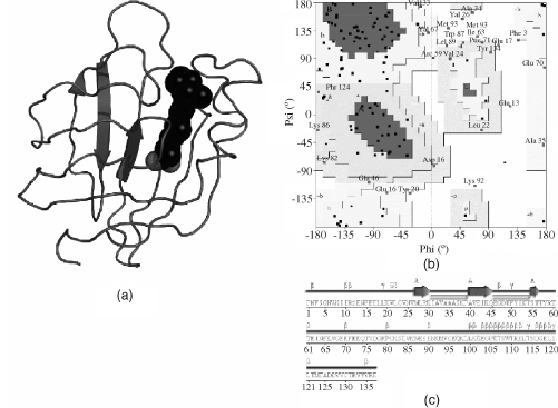
One feature that makes the Ramachandran plot such a powerful indicator of protein structure quality is that it is difficult to fool (unless one does so intentionally by, say, restraining f-y values during structure refinement as is sometimes done for NMR structures). This reliability was demonstrated by Gerard Kleywegt in Uppsala who once attempted to deliberately trace a protein chain backward through its electron density to see whether it would refine and give the sorts of quality indicators that could fool people into believing it to be a reasonable model (Kleywegt and Jones, 1995). Of the parameters that he tried to fool, the two that seemed least gullible were the R_free factor mentioned above, and the Ramachandran plot. Figure 14.10 shows this backward-traced model, together with its Ramachandran plot and secondary structure diagram (referred to later). The Ramachandran plot looks most unhealthy, with several residues in disallowed regions and no significant clustering in the most highly favored regions. The structure itself can be found in the PDBsum database under its fake PDB code of “fake”: http://www.ebi.ac.uk/pdbsum/fake.

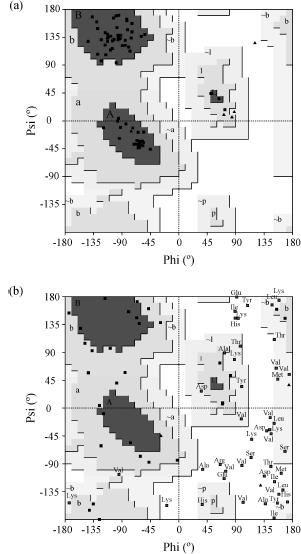
A simple measure of the overall “quality” of a model can be derived from the plot by computing the percentage of residues in the most favorable, or “core” regions. (Glycines and prolines are excluded from this percentage because of their unique distributions of available ø-ψ combinations.) Using the core regions shown in Figure 14.9, which are defined by the PROCHECK program (see below), one generally finds that the atomic resolution structures have well over 90% of their residues in these most favorable regions. For lower and lower resolution structures, this percentage drops, with the structures solved to 3.0-4.0 Atending to have a core percentage around 70%. NMR structures also show increasing core percentage with increasing experimental information. However, NMR structures can have relatively good side chain positions even with a poor core percentage as NMR data restrain side chains more strongly than the backbone because of the large number of side chain protons.

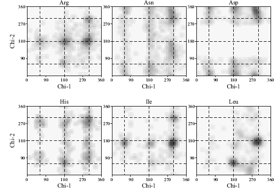
Side Chain Torsion Angles. Like its main chain, a protein’s side chains also have preferred conformations for their torsion angles. These conformations are known as rotamers and again are a result of steric hindrance making some conformations inaccessible. The side chain torsion angles are labeled χ₁, χ₂, χ₃, and so on. The first of these, χ₁, is defined as the torsion angle about N-C^α-C^β-A^γ, where A^γ is the next atom along the side chain (for example, in lysine the A^γ atom is C^γ). The next, χ₂, is defined as C^α C^β-A^γ-A^δ, and so on. The χ₁ and χ₂ distributions are both trimodal with the preferred torsion angle values being termed gauche-minus (+ 60°), trans (+180°), and gauche-plus (—60°). A plot of χ₂ against χ₁ for each residue has 3 x 3 preferred combinations, although the strength of each depends very much on the residue type. Figure 14.11 shows some examples of the χ₁-χ₂ distributions for different amino acid types.

Like the Ramachandran plot, a plot of the χ₁-χ₂ torsion angles can indicate problems with a protein model as these, like the ø and ψ torsion angles, tends not to be restrained during refinement. Also, like the Ramachandran plot, the clustering in the most favorable regions on the χ₁-χ₂ plot becomes tighter as resolution improves (EU 3D Validation Network, 1998). For example, the standard deviation of the χ₁ torsion angles about their ideal position tends to be around 8° for atomic resolution structures and can go as high as 25° for structures solved at 3.0 A. Similarly, the corresponding standard deviations for χ₂ tend to be 10° and 30°, respectively.

Bad Contacts. Another good check for structures to be wary of is the count of bad and unfavorable atom-atom contacts that they contain. Too many and the model is likely to be a poor one.

The simplest checks are those that merely count “bad” contacts. A bad contact is where two nonbonded atoms have a center-to-center distance that is smaller than the sum of their van der Waals radii. The check should be applied not only to intraprotein contacts within the given protein structure, but, for X-ray crystal structures, also to atoms from molecules related by crystallographic, and noncrystallographic symmetry.

More sophisticated checks consider each atom’s environment and determine how happy that atom is likely to be in that environment. For example, the ERRAT program (Colovos and Yeates, 1993) counts the numbers of nonbonded contacts, within a cutoff distance of 3.5 Å, between different pairs of atom types. The atoms are classified as carbon (C), nitrogen (N), and oxygen (O)/sulfur, so there are six distinct interaction types: CC, CN, CO, NN, NO, and OO. If the frequencies of these interaction types differ significantly from the norms (as obtained from well-refined high-resolution structures), the protein model may be somewhat suspect. Using a 9-residue sliding window and obtaining the interaction frequencies at each window position can locate local problem regions.

One level up in sophistication is the DACA method (Vriend and Sander, 1993) that is implemented in the WHAT IF (Vriend, 1990) and WHAT_CHECK (Hooft et al., 1996) programs. DACA stands for Directional Atomic Contact Analysis and compares the 3D environment surrounding each residue fragment in the protein with normal environments Computed from a high-quality data set of protein structures. There are 80 different main chain and side chain fragment types. The environment ofeach is essentiallythe count ofdifferent nonbonded atoms in each 1Å x 1Å x 1Å cell of a16Å x 16Å x 16Å cube surrounding the fragment.

A similar approach is used in the ANOLEA program (Atomic Non-Local Environment Assessment) that calculates a “nonlocal energy” for atom-atom contacts based on an atomic mean force potential (Melo and Feytmans, 1998). A relative newcomer to the field, which has become quite popular, is MolProbity (Lovell et al., 2003) that performs a detailed all-atom contact analysis within the given structure. The structure must include hydrogens so, where it doesn’t, a first step in the analysis is the addition and full optimization of all hydrogen atoms, both polar and nonpolar. Chapter 15 provides a more detailed description of the methodology of this program.

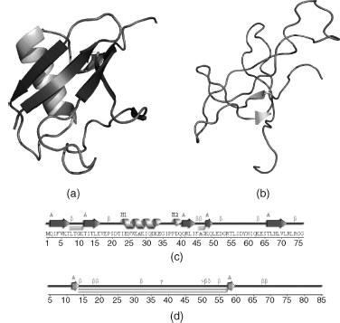
Secondary Structure. Occasionally, the model of a protein structure is so bad that one can tell immediately from its secondary structure. Most proteins have around 50-60% of their residues in regions of regular secondary structure, that is, in α-helices and β-strands. However, if a model is reallypoor, the main chain oxygen and nitrogen atoms responsible for the hydrogen bonding that maintains the regular secondary structures can lie beyond normal hydrogen bonding distances; so the algorithms that assign secondary structure (Chapter 19) may fail to detect some of the α-helices and β-strands that the correct protein structure contains. Figure 14.12 gives an example of the secondary structure contents for a typical protein and for the protein that had the poor Ramachandran plot in Figure 14.9b. The backward-traced protein at http://www.ebi.ac.uk/pdbsum/fake, mentioned above, also has very low secondary structure content (Figure 14.10c).

Other Parameters. Other parameters that can be used to validate protein structures include counts of unsatisfied hydrogen bond donors and hydrogen bonding energies as computed by the WHAT_CHECK program mentioned below (Hooft et al., 1996). Some programs—Prosa, Verify3D, and HARMONY—use knowledge-based potentials of some sort to assess how “happy” each residue is to be in the local environment that it finds itself in the current model. Very many unhappy residues make for a sad structure overall.

C-Alpha Only Structures. As of August 2007, there were around 274 structures in the PDB (out of over 45,000) containing one or more protein chains for which only the C^α coordinates had been deposited. The deposition of C^α-only coordinate sets is usually done where the data quality has been too poor to resolve more of the structure. This was common in the early days of protein crystallography but nowadays only tends to be done for very large structures, such as the recently determined structure of a 50s ribosomal subunit at 3.5 A(PDB code 1XBP; Schrunzen et al., 2004).

The standard validation checks are of no use for such models, lacking as they are in so much of their substance. However, there is an equivalent to the Ramachandran plot for these structures (Kleywegt, 1997). The parameters plotted are the C^α-C^α-C^α-C^α torsion angle as a function of the C^α-C^α-C^α angle for every residue in the protein. As with the Ramachandran plot, there are regions of this plot that tend to be highly populated, and others that appear to be “forbidden.” So a structure with many outliers in the forbidden zones should be treated with caution. The checks are incorporated in the STAN Web server (see later).

Nucleic Acids

Finding validation tools for DNA and RNA is trickier than for proteins. The PDB’s validation tool, AutoDep Input Tool (ADIT), incorporates a program called NuCheck (Feng, West-brook, and Berman, 1998) for validating the geometry of DNA and RNA. Binary versions of the ADIT package are included in the PDB Validation Suite (see Table 14.1).

A program specifically developed for checking the geometry of RNA structures, but which can also be used for DNA structures, is MC-Annotate (Gendron, Lemieux, and Major, 2001). It computes a number of “peculiarity factors,” based on various metrics including torsion angles and root-mean-squared deviations from standard conformations, which can highlight irregular regions in the structure that may be in error or merely under strain.

TABLE 14.1. Freely Available Programs for Checking Structure Coordinates Program name Reference URL

Program name	Reference	URL
ERRAT	Colovos and Yeates (1993)	www.doe-mbi.ucla.edu/People/Yeates/
		Gallery/Errat.html
HETZEa	Kleywegt and Jones (1998)	alphα2.bmc.uu’s e/usf/xutil.html
MC-Annotateb	Gendron et al. (2001)	www-lbit.iro.umontreal.ca/
		mcannotate-simple
MolProbity	Lovell et al. (2003)	molprobity.biochem.duke.edu
NUCheckb	Feng, Westbrook, and	See PDB Validation Suite below
	Berman (1998)
PDB Validation Suite	Westbrook et al. (2003)	sw-tools.pdb.org/apps/VAL
PROCHECK	Laskowski et al. (1993)	www.biochem.ucl.ac.uk/_roman/
		procheck/procheck.html
PROCHECK-NMR	Laskowski et al. (1996)
	www.biochem.ucl.ac.
	uk/_roman/
	procheck_nmr/
	procheck_nmr.html
Prosa 2003	Sippl (1993)	prosa’s ervices.came’s bg.ac.at/download/
		download.php
WHAT_CHECK	Hooft et al. (1996)	swift.cmbi.ru.nl/gv/whatcheck

^aFor hetero compounds only.

^bFor RNA and DNA only.

Hetero Groups

The geometry of hetero compounds, as deposited in the structures in the PDB tends to be of widely varying quality (Kleywegt et al., 2003). This is because, while there are well-established libraries giving standard bond lengths and bond angles for use in refinement of proteins and nucleic acids, there can be no equivalent for the wide variety of small ligand molecules that can bind to them. For any new ligand molecule, the target bond lengths and angles need to be individually compiled from scratch, based on its atom types and bond orders. This requires a thorough understanding of the molecule’s chemistry, so errors in the target values do occur. The PRODRG server (http://davapc1.bioch.dundee.ac.uk/programs/prodrg) can help reduce the effort involved and reduce the risk of errors (Schuttelkopf and van Aalten, 2004).

The HETZE program (Kleywegt and Jones, 1998) is one of the few validation methods that checks various geometrical parameters of the hetero compounds associated with PDB structures. These include bond lengths, torsion angles, and some virtual torsion angles, the information principally coming from the small-molecule structures in the Cambridge Structural Database (Allen et al., 1979).

SOFTWARE FOR QUALITY CHECKS

There are a large number of freely available programs that can perform the sorts of quality checks described above on proteins, nucleic acids, and hetero compounds. Table 14.1 lists a selection of these, with URLs giving links to their download information. The most commonly used programs are described below.

PROCHECK

The PROCHECK program (Laskowski et al., 1993), although now quite long in the tooth, is still commonly used for checking the quality of protein structures. It produces a number of plots in PostScript format, including Ramachandran plots, both for the protein as a whole and for each type of amino acid; χ₁-χ₂ plots for each amino acid type; main chain bond lengths and bond angles; secondary structure plot; deviations from planarity of planar side chains; and so on. Parameters that deviate from the norm are highlighted. The program has been incorporated into the PDBsum database (see later) and so its analyses are available for all PDB entries, including the obsolete ones. A version specifically for NMR, and other, ensembles is called PROCHECK-NMR (Laskowski et al., 1996) and provides plots that compare the various stereochemical parameters across all the models of the ensemble.

WHAT_CHECK

The WHAT_CHECK program (Hooft et al., 1996) is a subset of Gert Vriend’s WHAT IF package (Vriend, 1990). It contains an enormous number of checks and produces a long and very detailed output of discrepancies of the given protein structure from the norms. It also includes the DACA method, mentioned above, for analyzing nonbonded contacts. Precomputed WHAT_CHECK results for all PDB entries can be found in the PDBREPORT database (see later).

PDB Validation Suite

The PDB’s own internal suite of validation programs is available for download from the RCSB Web site as executable binaries (see Table 14.1). Although principally aimed at experimentalists preparing their models for deposition, it can also be used for validating otherstructural models. Where the corresponding experimental data are available, thesewill be included in the validation checks.

Other Programs

There are a numberofotherprograms available, whichperform avarietyofdifferentchecks on a given structure (see Table 14.1). Prosa 2003, the successor to Prosa II (Sippl, 1993), scores a protein structure using knowledge-based potentials representing atom-pair and protein-solvent interactions, as determined from a data set of known protein structures. The Verify3D program (Bowie et al., 1991) considers the environment of each residue in the 3D structure in terms of secondary structure type, buried surface area, and fraction of side chain area covered by polar atoms. A similar approach is given by HARMONY (Pugalenthi et al., 2006). The TAP program (Tosatto and Battistutta, 2007) validates the local torsion angles from propensities computed from known protein structure models. PROVE compares atomic volumes against a set of precalculated standard values (Pontius, Richelle, and Wodak, 1996). Volumes are calculated using Voronoi polyhedra to define the space that each atom occupies by placing dividing planes between it and its neighbors. The ERRAT and MolProbity programs have already been mentioned. Some programs are also available as Web servers (see later) and some are only available via Web servers (i.e., cannot be downloaded for local use).

QUALITY INFORMATION ON THE WEB

Much of the information given by the above packages is readily available on the Web, so one can often get it without installing and running any of the software itself. Several sites provide precomputed quality criteria for all existing structures in the PDB. Other sites allow you upload your own PDB file, via your Web browser, and will run their validation programs on it and provide you with the results of their checks.

PROCHECK Analyses in PDBsum

The PDBsum Web site at http://www.ebi.ac.uk/pdbsum (Laskowski, Chistyakov, and Thornton, 2005) provides numerous structural analyses ofall PDB structures. This includes the full PROCHECK output and a mini-Ramachandran plot for all entries containing one or more protein chains. Moving the mouse over the mini-Ramachandran pops up a full-sized version that can give an at-a-glance idea of the likely quality of the structural model in question. It is possible to obtain the PDBsum analyses, including full PROCHECK results, for structures not in the PDB using the Generate button on the PDBsum home page that returns the results on a password-protected set of pages.

PDBREPORT-WHAT_CHECK Results

The PDBREPORT database (http://swift.cmbi.ru.nl/gv/pdbreport) gives a precomputed WHAT_CHECK report for any structure in the PDB. The report is a detailed listing (supplemented by an even more detailed listing called the Full report) of the numerous analyses that have been precomputed using the WHAT_CHECK program. These include space group and symmetry checks, geometrical checks on bond lengths, bond angles, torsion angles, proline puckers, bad contacts, planarity checks, checks on hydrogen bonds, and more, including an overall summary report intended for users of the model.

RCSB Geometry Analyses

The RCSB Web site (http://www.pdb.org) also has geometrical analyses on each entry, consisting of tables of average, minimum and maximum values for the protein’s bond lengths, and bond angles and dihedral angles. Unusual values are highlighted. It is also possible to view a backbone representation of the structure in RasMol colored according to the “Fold Deviation Score”—the redder the coloring, the more unusual are the residue’s conformational parameters.

The Uppsala Electron Density Server (EDS). For X-ray crystal structures that have been deposited in the PDB together with their experimental data, the Uppsala Electron Density Server (EDS) at http://eds.bmc.uu.se (Kleywegt et al., 2004) provides useful information on the local quality of the structure. For example, the plot of the real space R-factor (RSR) shows how well each residue fits its electron density. Other useful plots include the occupancy-weighted average temperature factor and a Z-score associated with the residue’s RSR for the given resolution. The tall spikes in these plots identify residues that are either particularly disordered or do not sit well within their electron density and so may need to be treated with caution. A particularly nice feature is that clicking on any residue in these plots pops up a window running a Java-based 3D viewer showing the model and electron density in the region of the residue.

Validation Servers on the Web

The servers described above provide quality information on structural models that are already in the PDB. To check the quality of a model that is not in the PDB, one can submit it to one of the validation servers listed in Table 14.2. Most of these validate protein structures and use programs that are freely available for in-house use (see Table 14.1). However, the servers can often be easier and more convenient to use, and of course save you from having to download and install the programs.

Some servers run individual programs while others run compilations of two or more programs. Of the individual programs, ANOLEA, ERRAT, HARMONY, MolProbity, Prosa 2003, TAP, and Verify3D have already been mentioned. The STAN (Structure Analysis) server generates a standard Ramachandran plot, a “C^α-Ramachandran” plot, a plot analyzing any nucleic acid chains, a check for possible misidentification of small cations as waters, and check for incorrect cz’s-peptide bonds. Volume, Area, Dihedral Angle Reporter (VADAR) is a compilation of over 15 different programs (Willard et al., 2003), including PROCHECK and WHAT_CHECK. The COLORADO3D server (Sasin and Bujnicki, 2004) includes ANOLEA, PROSA, PROVE, and Verify3D, while the JCSG server includes PROCHECK, WHAT_CHECK, ERRAT, and PROVE. Finally, the PDBsum Generate server, which is not strictly speaking a validation server, generates a complete password-protected PDBsum analysis of any uploaded PDB file, including a full PROCHECK output.

TABLE 14.2. WWW Servers for Checking Uploaded Structure Coordinates Online

Server Name	Reference	URL
ANOLEA	Melo and Feytmans (1998)	protein.bio.puc.cl/cardex/
		servers/anolea
COLORADO3D	Sasin and Bujnicki (2004)	asia.genesilico.pl/colorado3d
EDS	Kleywegt et al. (2004)	eds.bmc.uu.se
ERRAT	Colovos and Yeates (1993)	nihserver.mbi.ucla.edu/
		ERRATv2
HARMONY	Pugalenthi et al. (2006)	caps.ncbs.res.in/harmony
JCSG Validation Server	Joint Center for Structural	www.jcsg.org/scripts/prod/
	Genomics	validation/sv_final.cgi
MolProbity	Lovell et al. (2003)	molprobity.biochem.duke.edu
PDBsum Generate	Laskowski et al. (2005)	www.ebi.ac.uk/thornton-srv/
		databases/pdbsum/upload.
		html
PDB Validation Server	Westbrook et al. (2003)	deposit.rcsb.org/validate
ProSA-Web	Wiederstein and Sippl (2007)	prosa.services.came.sbg.ac.at/
		prosa.php
STAN	Kleywegt and Jones (1996),	xray.bmc.uu.se/cgi-bin/gerard/
	Kleywegt (1997)	rama_server.pl
TAP	Tosatto and Battistutta (2007)	protein.cribi.unipd.it/tap
Verify3D	Bowie et al. (1991)	nihserver.mbi.ucla.edu/
		Verify_3D
VADAR	Willard et al. (2003)	redpoll.pharmacy.ualberta.ca/
		vadar

CONCLUSIONS

The main aim of this chapter has been to impress upon you that the macromolecular structures that form the very foundation of Structural Bioinformatics are not all of the same quality and can undermine those foundations if not carefully selected. All structures are just models devised to satisfy data obtained experimentally. As such, they will contain errors, both systematic and random. Some structures have been found to be seriously incorrect— that is, they are inaccurate models of the molecules they represent and in many cases have been replaced by more accurate models. Most structures are reasonably accurate but inevitably contain random errors, as is symptomatic of any experimental measurement. The quality of structures as a whole has improved over the past few years and this trend is expected to continue. However, determining which is a good structure and which is not is still not clear. Even traditional measures such as the resolution and R-factor for X-ray structures, and number of restraints for NMR structures do not always separate the good from the bad. Most often, other quality measures need to be taken into account when selecting a good data set.

The chapter has surveyed the information available, and some of the additional tests that can be performed to ensure that the reliability of any of the structures used is consistent with the conclusions to be drawn from them.

ACKNOWLEDGMENTS

Thanks to Drs Mark Williams and Gert Vriend for their valuable comments on the text of this chapter.