19
SECONDARY STRUCTURE ASSIGNMENT
The Task. When looking at how chains of amino acids in proteins are ordered, we notice regular macro elements in the 3D structure of practically all known structures: helices and strands (see Chapter 2). These structures were coined protein secondary structure by Linderstrøm-Lang (1952) in the context of a protein’s primary, tertiary, and quaternary structural definitions. There is no unique inherent physical characteristic to systematically assign secondary structure from 3D coordinates. Instead there are many different assignment schemes, each constructed to reflect one or more aspects of protein structure. Here we will address these aspects, the assignment schemes, and how they have been used to study proteins.
Aspects Reflected in Secondary Structure Assignments. When protein secondary structure is assigned, the complexity of the all atom 3D structure is reduced dramatically. This level of abstraction is obtained by choosing as determinants for the assignment such aspects as physical interaction energies (e.g. H-bonds and van der Waals), geometrical idealization (e.g. idealized cylinder or Cα-distance masks) and/or other structural descriptions optimized to reflect appealing characteristics (e.g. expert assignment, invariance upon thermal fluctuations or predictability). Another generic aspect of all methods is that they assign secondary structure based on residue independent aspects.
Notation. When treating protein secondary structure, we will use the terms: state, class, and regular secondary structure. In the literature, these are not used consistently so we refer to the following notation: states are the types of secondary structures defined by a particular method, for example, G refers to 310-helix in the dictionary of secondary structure of proteins (DSSP); classes are the groups of similar states, for example, G, H and I all describing helices in DSSP; regular secondary structure are all the states belonging to a direct secondary structure assignment. Note that nonregular structure thus refers to the remaining states, which on occasion go by names such as random coil or loop. Super secondary structure refers to the relative spatial distances and orientations between two or more secondary structure elements.
Usage of Secondary Structure. The application of secondary structure assignments is very diverse and covers many areas of protein analyses, most noticeably, within structure inspection (Chapters 14 and 15), visualization (see Chapter 9) and the related task of structure comparison and classification (see Chapters 16, 17 and 18). Secondary structure has also been employed in protein modeling and structure prediction (see Chapter 29), as well as in studies of protein folding, dynamics, interactions, and function. The one-dimensional nature of the secondary structure description has furthermore been used in sequence alignment. Some applications will be treated in more detail below after the assignment methods have been described.
History: From Expert to Automatic Assignment of Protein Secondary Structure. Pauling and colleagues correctly predicted the idealized protein secondary structures of α-helices (Pauling et al., 1951), π-helices (Pauling et al., 1951), and of β-sheets (Pauling and Corey, 1951) based on intra-backbone hydrogen bonds. Five decades later, we know that on an average about half of the residues in proteins participate in helices or sheets (Berman et al., 2000). Pauling and colleagues incorrectly predicted that 310-helices would not occur in proteins due to unfavorable bond angles; approximately 4% of the residues are observed in this conformation (Andersen, 2001). Initially, crystallographers assigned secondary structure by eye from the 3D structures. This was the only way to assign secondary structure at that time. However, it lacked consistency since experts occasionally disagreed. This was particularly problematic when comparing secondary structure predictions and was actually the primary objective for Kabsch and Sander (1983a), and Kabsch and Sander (1983b) to automate the assignment in their DSSP program. Originally developed to improve secondary structure prediction, DSSP has remained the standard in the field, most popular for its relatively reliable assignments. Curiously, the prediction method for which Kabsch and Sander created to address this issue was never published.
Experimental Investigations of Protein Secondary Structure. The structure of a protein can be determined at various levels of precision and timescale. X-ray crystallography (see Chapter 4) is widely used and generally provides a static snapshot with all atom resolution, whereas NMR (see Chapter 5) furthermore can measure dynamic motion of proteins in solution, but not below the millisecond regime (Doerr, 2007). Optical spectroscopy is a much faster technique and has been used to inspect H-bond dynamics at a picosecond time scale for a small β-turn peptide (Kolano et al., 2006). In particular circular dichroism (CD) and Raman spectroscopy are used to characterize overall protein secondary structure dynamics in solution, since the helix and sheet structures give strong characteristic spectra which are highly correlated with X-ray data (Tetin et al., 2003; Janes, 2005; Lees et al., 2006). This allows the rapid assessment of conformational changes resulting from ligand binding, macromolecular interactions, and so on, and conformational assessment of natively unfolded proteins (Pelton and McLean, 2000; Maiti et al., 2004). Spectroscopy resolution can be further enhanced with residue-specific isotope labeling, for example, to dissect the conformation of helical peptides at the residue level (Decatur, 2000; Fesinmeyer et al., 2005). Attempts have been made to determine the protein secondary structure and stability by mass spectrometry (Villanueva et al., 2002), but the specific technique presented is not likely to be a valuable conformational probe (Beynon, 2004).
The hydrogen bond is used by many methods to describe and assign protein secondary structures, so we will introduce this concept and some definitions employed. Using the hydrogen bond spurs from the notion of assigning secondary structure based on the local energy gained in stabilizing the polypeptide chain in a given conformation. Following this notion, the energetic calculation can also be extended to the rest of the protein backbone atom interactions by calculating electrostatic and van der Waals interaction energies, described here as the backbone-backbone interaction energy.
Likewise, mathematical concepts are applied to secondary structure assignment. These may be basic geometrical objects, which can be readily comprehended (e.g. a straight line or cylinder) or may require some introduction as done for Voronoï tessellation presented here.
Hydrogen Bond Energy
Pauling (1939) established the hydrogen bond as an important principle in chemistry. The rich network of hydrogen bonds in water creates a very particular environment in which polar molecules participate, while nonpolar molecules disrupt the network of hydrogen bonds. This results in missing water-water hydrogen bonds and therefore a relative energy cost compared to the hydrogen bonded case (4 kcal/mol for isoleucine and leucine when compared to glycine (Creighton, 1993)). This energy cost is in the order of two hydrogen bonds (hydrogen bonds are in the range of —2 kcal/mol) and can be avoided or minimized by packing via agglomerating nonpolar molecules, thereby resulting in the hydrophobic effect.
The packing of nonpolar residues in the core is believed to be the main driving force in tertiary structure formation of proteins, while the specific secondary structures are governed by intramolecular hydrogen bonds (Hvidt and Westh, 1998). Packing the nonpolar residues in the core also means burying the polar backbone atoms and breaking the water-backbone hydrogen bonds. To avoid this heavy energetic cost, the polarities are paired (forming hydrogen bonds) in the protein core, thus fixing the protein conformation. If instead the protein backbone were nonpolar, the protein core elements would then be free to move around, thus leading to a highly dynamic protein structure and thereby preventing the protein from functioning reliably and efficiently.
Approximately 90% of the backbone C=O and NH groups participate in hydrogen bonds (Baker and Hubbard, 1984). Using the Coulomb hydrogen bond definition (see below), we found that approximately 62% of the backbone C=O and NH groups participate in intra-backbone hydrogen bonds (Andersen, 2001). Pauling defined secondary structure by the intra-backbone hydrogen bonds, and this has later become the prevalent means of assigning secondary structure. Thus, for simplicity, we refer to intra-backbone hydrogen bonds when using the term “hydrogen bond”.
Angle-Distance Hydrogen Bond Assignment
There are many different angles and distances that can be measured and used to identify the hydrogen bond. Baker and Hubbard (1984) assigned hydrogen bonds according to the inter-atom angle NHO = q and distance rHO in the hydrogen bond. A hydrogen bond is assigned when
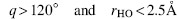
This is similar to other rigid distance and angle constraints published (Bordo and Argos, 1994; Jeffrey and Saenger, 1994), and can be simplified further by considering only the donor-acceptor distance, that is, in this case hydrogen bonds are assigned when rHO < 3.5 Å. Although a rather crude way of assigning hydrogen bonds, it has sufficed for several decades and is still being used.
Coulomb Hydrogen Bond Energy Calculation
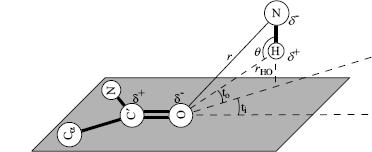
One way of finding hydrogen bonds is by calculating the Coulomb energy in the bond, as applied in DSSP (see below) focusing on the electrostatic attraction (Figure 19.1). The Coulomb energy for the attraction and repulsion is given by
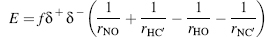
where f = 332 Å kcal/(e2 mol) is the dimensional factor, and δ+ = 0.20e and δ-=-0.42e are the polar charges given in units of the elementary electron charge e. A cut-off level has been set for the weakest acceptable hydrogen bond so that the resulting energy is bound by E < —0.5 kcal/mol in DSSP. In practice, the hydrogen atom position is usually not given in periplasmic binding protein (PDB files requiring an extrapolation. For example, the hydrogen atom position that is needed to calculate the two distances rOH and rHC’ in Equation 19.1 is usually not given in the PDB files. DSSP circumvents this problem by using an approximate position, assuming that the covalent bond between O=C’ is parallel to the covalent N—H bond adjacent to the same polypeptide bond. The direction of the O=C’ vector is kept while its length is set to 1 Å, that is, the length of the N—Hbond(Creighton, 1993). The position of the H-atom is extrapolated using the direction of the C’=O vector when starting out from the position of the N-atom. These approximations made by DSSP simplify the calculation of the H-atom position and appear to be rather accurate despite the assumptions that were being made. When compared to the original bond angles and distances (Creighton, 1993), we found the DSSP approximation to yield an average error around 0.07 Å (Andersen, 2001). The assumption of the trans-peptide bond, giving rise to the rigid peptide plane, was used by DSSP as well as our tests. Partitioning ab initio energy calculations of the hydrogen bond into classical components showed that about 75% is electrostatic (Coulombic) and less than 5% comes from polarization and charge transfer, for moderate strength bonds (Jeffrey and Saenger, 1994). Note that the Coulomb energy term does not incorporate atom-atom repulsion to penalize steric clashes and does not give rise to a characteristic hydrogen bond length.
Figure 19.1. Distances used to calculate the Coulomb hydrogen bond energy.

Empirical Hydrogen Bond Energy Calculation
An empirical hydrogen bond energy calculation can be derived from the hydrogen bond geometry in crystal structures or from polypeptides, peptides, amino acids, and small organic compounds (Boobbyer et al., 1989; Wade et al., 1993) as applied in secondary STRuctural IDEntification method (STRIDE) (see below). The total energy Ehb depends on the NO distance energy Er, (reflecting optimal atom distance and atom boundary) and on three bonding angles through the expressions Ep and Et (reflecting favorable hydrogen bond angles extrapolated from electron orbital interactions):
(19.2)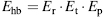
The distance dependency energy Er is similar to the Lennard-Jones potential for the van der Waals interaction, but uses powers of eight and six instead of 12 and six. Thus reducing the slope of the atom-atom superposition term, whereby the penalty for superpositions is more lenient towards experimental inaccuracies in atom position determination.
(19.3)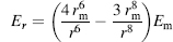
where r is the NO distance, rm the optimal distance, and Em the optimal energy. For intra-backbone hydrogen bonds rm — 3.0 Å and Em =— 2.8 kcal/mol is used. The two angular dependent terms are
(19.4)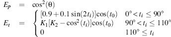
where the angles θ, ti, and t0 are specified in Figure 19.2.
Backbone-Backbone Interaction Energy
The Coulomb and van der Waals interaction energy calculations can also be applied
to all backbone atom interactions (i.e. involving the atoms N, Cα,C’,O,HN and Hα) as applied in β-spider (see below),
thereby covering the two potential backbone hydrogen bonds formed between two residues (described
above), as well as the Cα—Hα O=C hydrogen
bond and the C=O... C=O dipole. This energy evaluation is calculated for
each atom pair  and subsequently summed
over all pairs between two residues
and subsequently summed
over all pairs between two residues  . has the same functional form as the Amber
force field (Cornell et al., 1995):
. has the same functional form as the Amber
force field (Cornell et al., 1995):
(19.5)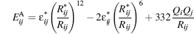
where is the energy between
atoms i and j with observed distance Rij (Å), mixing rules  , polar charges Qi, Qj, and
optimal distance
, polar charges Qi, Qj, and
optimal distance  . The optimal distance,
mixing rules, and polar charges were taken from Amber. In the special cases of glycine and proline, the
backbone constellation has been adjusted accordingly by adding another Hα
and removing the HN, respectively. In β-spider the hydrogen atom positions
were extrapolated geometrically from the N, Cα,C’ and O coordinates using
bond lengths, valence, and torsion angles from Amber (Cornell et al., 1995).
. The optimal distance,
mixing rules, and polar charges were taken from Amber. In the special cases of glycine and proline, the
backbone constellation has been adjusted accordingly by adding another Hα
and removing the HN, respectively. In β-spider the hydrogen atom positions
were extrapolated geometrically from the N, Cα,C’ and O coordinates using
bond lengths, valence, and torsion angles from Amber (Cornell et al., 1995).
(19.6)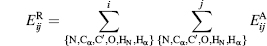
Figure 19.2. Angles and distances defining the empirical hydrogen bond. Note: Figure similar to the one in Frishman and Argos (1995).
Voronoï Tessellation for Geometrical Residue Partitioning
By geometrically deriving a polyhedron around the Cα of each residue using Voronoï tessellation a new definition of contact maps is described. This is very informative about the relative packing of residues and has been applied to assign secondary structure by VoTAP (see below). Each Cα is contained within a Voronoï cell, which is determined by Delaunay tetrahedral decomposition. This is a unique decomposition with nonoverlapping cells that only contain one Cα atom each and where all internal space inside the protein is contained within a cell as shown in Figure 19.3.
Converting Secondary Structure States to Three Classes
Several secondary structure assignment methods are presently available, but DSSP continues to be the most widely used method followed by STRIDE. In fact, most prediction methods are based on DSSP assignments. Typically, the eight DSSP states are converted into three classes using the following convention: [GHI] → h, [EB] → e, [TS“”] → c, which reads 310-, α-, π-helices are grouped into one helix class; extended β-sheets and β-bridges are grouped into one sheet class; and the remaining secondary structure states: turn, bend and “not assigned” are grouped into one coil class.
Usually, 310-helices and β-bridges constitute short secondary structure segments that have some structural similarity to α-helix and β-strand, respectively. However, they do have different sequence characteristics. Prediction methods, in general, are more precise in the core of regular secondary structure segments than at the termini (Rost, 1995; Cuff and Barton, 1999). Thus, 310-helices and β-bridges are more difficult to predict than α-helices and β-strands. Therefore an alternative conversion that has been used more recently yields a seemingly higher level of prediction accuracy: [H] → h, [E] → e, [GIBTS“”] → c.
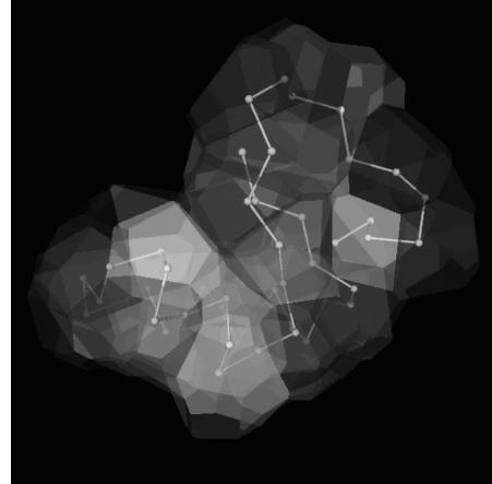
Figure 19.3. Voronoï tessellation partitions the protein space into polyhedra surrounding the Cα atom of each residue (Dupuis et al., 2004). Aunique Cα atom contact map can thus be defined as the polyhedra sharing a contact surface. The example shown is Crambin (Teeter, 1984; PDB: 1CRN) visualized from an angle similar to the one employed in Figure 19.9, using the voro3D tool made available to the community by Frank Dupuis.
ASSIGNMENT METHODS
DSSP: H-Bond Pattern-Based Assignment
The so-called DSSP by Kabsch and Sander (1983a) performs its sheet and helix assignments solely based on the backbone-backbone hydrogen bonds. The DSSP method defines a hydrogen bond when the bond energy is below —0.5 kcal/mol from a Coulomb approximation of the hydrogen bond energy (see Section “Secondary Structure Concepts”). The structure assignments are defined such that visually appealing and unbroken structures result. In case of overlaps, α-helix is given first priority, followed by β-sheet. This procedure does not affect the Coulomb approximation, rather the realization of ’’unbroken structures’ addresses the step from individual hydrogen bonds to assigning macrostructures to groups of such bonds (Figure 19.4).
An α-helix assignment (DSSP state “H”) starts when two consecutive amino acids have i → i - 4 hydrogen bonds, and ends likewise with two consecutive i → i — 4 hydrogen bonds. This definition is also used for 310-helices (state “G” with i → i + 3 hydrogen bonds) and for r-helices (state “I” with i → i + 5 hydrogen bonds) as well. The helix definition does not assign the edge residues having the initial and final hydrogen bonds in the helix. A minimal size helix is set to have two consecutive hydrogen bonds in the helix, leaving out single helix hydrogen bonds, which are assigned as turns for all three helices (state “T”).
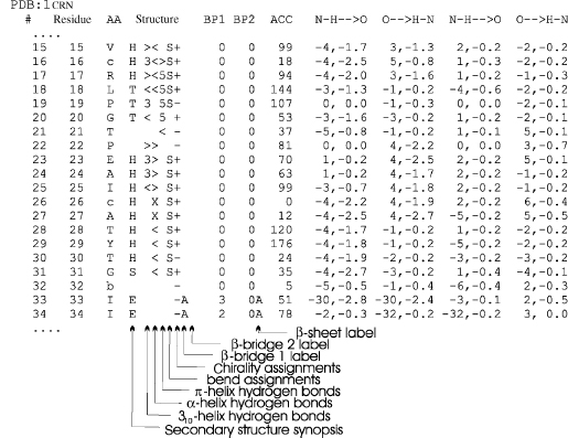
Figure 19.4. Explanation of DSSP output example segment from Crambin (Teeter, 1984). The first two columns contain the unique DSSP residue number and the corresponding PDB residue number. The third column (here empty) indicates the chain identifier if there are multiple chains. Then follows the amino acid “AA” in one letter codes (Note: lowercase letters are all cysteines, in orderto match up cysteine-bridges, for example, residue 16 has a disulfide bond to residue 26). The “Structure” section starts with the secondary structure synopsis (HBEGITS listed in order of priority in case of overlaps) and is followed by helix hydrogen bond indications for 310-, a-, and rc-helix hydrogen bonds, where “>” indicates an acceptor, “<” a donor and “X” both. The bend and chirality are each given a column followed by the (3-bridge label columns (lower case labels are parallel (3-bridgesand uppercase are antiparallel). The DSSP numbers of their partners are written in the“BP1”and “BP2” columns. Each p-sheet is also given a label (independent of the p-bridge labels) indicated in the adjacent column. The “ACC” column contains the solvent accessible surface measured in Å2 by estimating the number of water molecules in contact with the present residue. The two strongest backbone-backbone hydrogen bonds are then listed, where “N-H → O” are donor hydrogen bonds and “O → H-N” acceptor hydrogen bonds. The format indicates the relative sequence position of the hydrogen bond partner followed by the energy in kcal/mol (e.g. “-5,-0.8” means that the partner residue’s DSSP number is 5 less than the present 1 and that the hydrogen bond energy is -0.8 kcal/mol. The DSSP output also contains the Cα coordinates, phi-psi angles and other angles which were left out in this figure due to limitations of space.
β-Sheet residues (state “E”) are defined as either having two hydrogen bonds in the sheet, or being surrounded by two hydrogen bonds in the sheet. This implies three sheet residue types: antiparallel and parallel with two hydrogen bonds or surrounded by hydrogen bonds. The minimal sheet consists of two residues at each partner segment. Isolated residues fulfilling this hydrogen bond criterion are labeled as β-bridge (state “B”). The recurring H-bonding patterns connecting the partnering strands in a β-sheet are occasionally interrupted by one or more so-called β-bulge residues. In DSSP these residues are also assigned as p-sheet “E” and may comprise up to four residues on one strand and up to one residue on the partnering strand. These interruptions in the β-sheet H-bonding pattern are only assigned as sheet if they are surrounded by H-bond forming residues of the same type, that is, either parallel or antiparallel. The remaining two DSSP states “S” and (space) indicate a bend in the chain and the unassigned/other state, respectively.
DSSPcont: Continuous DSSP Assignment Reflecting Protein Motion
The aim of the continuous assignment was to reflect the structural variability due to thermal motion in a way so that regions which do not vary upon thermal motion have crisp assignments (almost discrete values), while regions which undergo thermal motion should reflect this in their continuous assignment and ideally reflect the occupancy of each secondary structure state. We estimated this by following the energy-based secondary structure assignment of DSSP and letting the strength of the hydrogen bond reflect thermal motion in the assignment (Andersen et al., 2002). This concept led us to develop a continuous extension of DSSP. This continuous assignment is based upon multiple runs of DSSP with different hydrogen bond thresholds. Then, we compiled a weighted average over the individual DSSP assignments to assign secondary structure to each residue. We determined the weights by applying the above criterion for “good” assignments starting with structural homologues from the FSSP (Holm and Sander, 1998) database. Inspecting the structural alignments in detail, we noted a number of possible reasons for observed structural differences:
1. Different solution composition, spatial grouping, and/or environment of the proteins.
2. Uncertainties/errors in the experimental structure determination setup.
3. Minor thermal fluctuations (even though mostly averaged out).
4. Local amino acid substitutions causing the structural change.
5. Insertions/deletions adjacent to the local stretch in question.
6. Nonlocal changes forcing a new local conformation.
7. Other less likely causes, for example, prion-like switching.
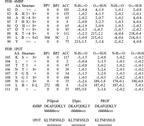
Our objective was a secondary structure assignment method de-emphasizing the effects of 1-3 while capturing differences caused by sequence changes. However, for structural alignments of homologues, we cannot separate these effects as illustrated by a comparison between two related structures: periplasmic binding protein (PDB: 4MBP; Quiochoet al., 1997) and putrescine binding protein (PDB: 1POT; Sugiyamaet al., 1996). The structural alignment was obtained from FSSP with a Z-score of 23.2 and an RMSD of 3.6 Aover 303 residues. We will focus on a small 10-residue segment (Figure 19.5a) that has spiraling structure (α-helix, 310-helix or turn) and a β-bridge at the penultimate position (Figure 19.5a). Based on the assignment alone one might characterize the differences as problems in the assignment process, since both segments have 310-helix hydrogen bonds over the entire stretch. On the contrary, 1POT has no a-helix hydrogen bonds resulting in the assignment of 310-helix. The results from three high-quality prediction methods (Figure 19.5b) suggest that the structural differences resulted from the sequence divergence. This means that the secondary structure assignments of the two segments should not necessarily be the same. This line of reasoning can be extended from short helices to short sheets and to the N- or C-terminal ends of helices and strands (caps).
Figure 19.5. DSSP assignments for similar structures: 4MBP and 1POT. (a) The DSSP assignment for two segments taken from two structurally similar proteins (periplasmic binding protein 4MBP: Quiocho et al., 1997, and putrescine binding protein 1POT: Sugiyama et al., 1996) illustrates that the observed differences between these segments may originate from sequence differences. The boxed letters shown in the column next to the amino acid sequence give the final DSSP assignment: G = 310-helix, H = α-helix, T = turn, B = β-bridge, and S = bend. The next column shows the hydrogen bonds (>: hydrogen bond acceptor, <: hydrogen bond donor and X: both), with indications of the hydrogen bond length, that is, i → i + (3,4) for 310 and α-helices, respectively. (b) All the predictions from PSIpred (Jones, 1999a; Jones, 1999b), SSpro (Baldi et al., 1999) and PROFphd (Rost, 1996) (see Chapter 29) correctly spot the α-helix signal in 4MBP, while missing this signal for 1POT. This may indicate that the altered sequence changed the structure significantly in this region. Here, “h” refers to the DSSP class helix (H or G) and “e” to the DSSP nonregular class. Note: The predictions are cut out from those for the entire protein.
Therefore, we chose to optimize the weights for DSSPcont based on the comparisons between different NMR models for the same protein.
Figure 19.6.Protein motion and secondary structure. Using one set of coordinates from an ensemble of NMR models, the continuous DSSP assignment reproduces the segments in proteins that experimentally had a high degree of motion due to thermal fluctuations in water. Protein motion has been independently measured by the order parameter 1-S2, by the tumbling of the N-H backbone bond-vector. 1-S2 is low when the amino acid is fixed as in the protein core, and it is high when the residue fluctuates. 1-S2 is shown versus the continuous DSSP assignment grouping helices (GHI) and strands (EB). The points are averages over a window segment of three consecutive residues; the line gives an average of helix/strand assignments. Source: Figure reproduced from Andersen (2001).

We found that the single residue RMSD between models of high-quality NMR structures correlated well with thermal fluctuations in water as independently measured by the order parameter. The resulting continuous DSSP assignments were constructed to reflect the differences between NMR models of the same protein, so that the assignments reflect segments with thermal fluctuations (Figure 19.6). This means that more the sequence segment fluctuates, the lower the probability for the assigned helix/sheet will become. Information of this type can also be obtained directly from crystal structures. Overall, we found that the continuous assignment of secondary structure reflected the average occupancy of secondary structure assignments. In particular, our continuous assignment for a single NMR structure is similar to the average obtained over all models.
STRIDE: H-Bond and phi/psi Angle-Based Assignment Mimicking Experts
The STRIDE by Frishman and Argos (1995) uses an empirically derived hydrogen bond energy (see Section “Secondary Structure Concepts”) and phi-psi torsion angle criteria to assign secondary structure. Torsion angles are given α-helix and β-sheet propensities according to how close they are to their regions in Ramachandran plots (see Chapter 2, Figure 19.6) (Ramachandran and Sasisekharan, 1968). The method fixes five internal parameters for α-helix and four for β-sheets. The parameters are optimized to mirror visual assignments made by crystallographers for a set of proteins. However, crystallographers often disagree in their assignment of secondary structure, which STRIDE aims to even out by averaging over many structures. Since the secondary structure categories have different parameters, their assignment thresholds are independent for the hydrogen bond and phi-psi torsion angles. By construction, the STRIDE assignments agreed better with the expert assignments than DSSP, at least for the dataset used to optimize the free parameters. In particular, the authors reported that every 11th β-sheet and every 32nd α-helix was more in register with the expert assignments for the data set used (Figure 19.7).
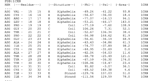
Figure 19.7. Explanation of STRIDE output. The STRIDE output for Crambin is shown to explain the format and for comparison to Figure. The format is simple and easily parsed, with “ASG” as the first word in the lines used for assignment. The residue columns comprise the three-letter amino acid code, the chain identifier (“-” for single chains), the PDB residue number and the STRIDE residue number, which starts from one for every new chain. The two structure columns contain the oneletter structure assignments (HGIEBbTC) and its short description. The columns with phi and psi are followed by the column with solvent accessibility (measured in Å2
Like DSSP, STRIDE assigns the shortest α-helix (“H”) if it contains at least two consecutive i → i + 4 hydrogen bonds. In contrast to DSSP, helices are elongated to comprise one or both edge residues if they have acceptable phi-psi angles, similarly a short helix can be removed if the phi-psi angles are unfavorable. This implies that hydrogen bond patterns may be ignored if the phi-psi angles are unfavorable. The sheet category does not distinguish between parallel and antiparallel sheets. The minimal sheet (“E”) is composed of two residues each in one of five possible hydrogen bond conformations, that is, two more than for DSSP. The dihedral angles are incorporated into the final assignment criterion as was done for the α-helix. β-Sheet bulges are accepted applying the same criterion as DSSP. Single residue sheets, that is, β-bridges are labeled as “B” for the three DSSP hydrogen bond conformations and as “b” for the remaining two. 310- (“G”) and π-helices (“I”) are implemented according to the DSSP scheme, but with the empirical hydrogen bond criterion. Turns are assigned according to the phi-psi angles of residue i + 1 and i + 2 as described in Wilmot and Thornton (1990). The “C” symbol is used whenever none of the above structure requirements is met.
STICK: Continuous Assignment Based on Line Segments
The standard method used to define line segments is to fit an axis through each secondary structure element (e.g. DEFINE). This approach has difficulties, with both inconsistent definitions of secondary structure and the problem of fitting a single straight line to a bent structure. STICK avoids these problems by finding a set of line segments independently of any external secondary structure definition (Taylor, 2001). This allows the segments to be used as a novel basis for secondary structure definition by taking the average rise per residue along each axis to characterize the segment. This practice has the advantage that secondary structures are described by a single (continuous) value that is not restricted to the conventional classes of α-helix, 310-helix, and β-strand. This latter property allows structures without “classic” secondary structures to be encoded as line segments that can be used in comparison algorithms. When compared over a large number of pairs of homologous proteins, the current method was found to be slightly more consistent than a widely used method based on hydrogen bonds.
Beta-Spider: Packing Energy Assignment
The stabilizing factors maintaining the secondary structure were used in β-spider
(Parisien and Major, 2005) as the primary parameters for assignment. This was done by calculating the
packing energy of the backbone interactions in the form of Coulomb electrostatic and van der Waals
forces (see Section “Secondary Structure Concepts”). For possible β-sheet interacting strands, the
packing energy was calculated for tri-peptide pairs and defined as “favored” if at least —5
kcal/mol (—1.67 kcal/mol per residue). This may seem as more than three times the interaction
energy required by DSSP H-bonds (—0.5 kcal/mol per residue), but the number of possible polar atom
interactions per residue has also tripled (two H-bond donors/acceptors and one dipole), and furthermore
the van der Waals energy is included. Two geometrical considerations are also used, which require that
the sheet residue pairs are maximally 6 A apart and; that the torsion  So, if Cαi and Cαy are aligned, the projected angle spanned between the two Cp must be less
than 90°, that is, point either towards each other or away from each other (glycine is exempted).
β-bulges up to three residues in length are also allowed within the sheet. In summary, a β-spider sheet
must contain at least one energetically “favored” tri-peptide pair and start/end with a residue pair
following the geometrical requirements and be at least two residues long. This setup increases the set
of tripeptide H-bonding motifs allowed within a β-sheet, resulting in approximately 11% and 6% increase
in number of motif matches for parallel and antiparallel sheets as compared to DSSP, respectively. At
present only a β-sheet assignment scheme has been published.
So, if Cαi and Cαy are aligned, the projected angle spanned between the two Cp must be less
than 90°, that is, point either towards each other or away from each other (glycine is exempted).
β-bulges up to three residues in length are also allowed within the sheet. In summary, a β-spider sheet
must contain at least one energetically “favored” tri-peptide pair and start/end with a residue pair
following the geometrical requirements and be at least two residues long. This setup increases the set
of tripeptide H-bonding motifs allowed within a β-sheet, resulting in approximately 11% and 6% increase
in number of motif matches for parallel and antiparallel sheets as compared to DSSP, respectively. At
present only a β-sheet assignment scheme has been published.
XTLsstr: Circular Dichroism Driven Assignment
The circular dichroism of a protein in the far ultraviolet range is determined principally by amide-amide interactions of the backbone (King and Johnson, 1999), which has driven the authors to develop a protein secondary structure assignment scheme: XTLsstr. The program calculates two backbone dihedral angles and three distances (two of which are simple two atom H-bond distances), which are used for the assignment. By visual inspection the authors have developed range definitions for each secondary structure (310-, α-helices, β-sheets and two turn types) that would be consistent with the amide-amide interactions observed in CD.
VoTAP: Residue Contact Assignment Based on Geometry
By first dividing the protein volume into residue specific polyhedra using Voronoï ’ tessellation, a residue contact map is automatically defined (Dupuis et al., 2004) (see Section “Secondary Structure Concepts”). This contact map is unique and does not depend on a distance threshold, here two residues are in contact if they share one face of their polyhedra. The contacts were divided into strong and normal contacts based on the contact surface area size in a residue specific manner, thus yielding three residue-residue contact designations 0,1, and 2 for no, normal, and strong contact, respectively. VoTAP assigns residues into the three overall classes helix (310, α and π), sheet (antiparallel, parallel, and β-bridge), and coil. The assignment was performed by fitting contact pattern statistics to the consensus assignment of DSSP, PSEA, DEFINE and STRIDE in two steps. The first step focuses on the diagonal of the contact matrix by comparing residue contact quintuplets. A lookup table for each quintuplet was created for the consensus assignment and a probability for each secondary structure class stored. A secondary structure class probability is subsequently assigned to each residue using a sliding window. In the second step the off-diagonal contacts are used to assign sheet residues if they follow the parallel or antiparallel β-plated sheet pattern. By VoTAP helices and sheets are constrained to be at least three residues in length.
DEFINE: Idealized Cα-Distance Mask-Based Assignment
The algorithm DEFINE (Richards and Kundrot, 1988) assigns secondary structures by matching Cα-coordinates with a linear distance mask of the ideal secondary structures. First, strict matches are found, which subsequently are elongated and/or joined allowing moderate irregularities or curvature. The algorithm locates the starts and ends of α- and 310-helices, β-sheets, sharp turns and omega-loops. With these classifications, the authors are able to assign 90-95% of all residues to at least one of the given secondary structure classes.
To assign α-helices the linear mask is matched with each row in the distance matrix of the query protein and the root mean square difference between the distances in the mask and the ones observed in the query protein is calculated as a measure of cumulative discrepancy. If a segment longer than four residues matches the mask within the allowed cumulative discrepancy limit (default ε = 1Å), and α-helix is assigned to the segment. Assigned α-helices are checked whether they start or end with a 310-helix, but individual 310-helices and p-helices are not investigated.
In order to assign β-sheets as a single category, the authors have applied a linear distance mask taken from ideal antiparallel sheets. The problems associated with backbone bend-ability inside sheets and curvatures in larger sheets have been “solved” by excluding nonrigid sheets from the definition. The minimum length of sheets is set to be four residues. According to Pauling’s definition of a p-sheet, each strand must pair to another strand to form a sheet. In contrast, DEFINE may assign unpaired strands.
P-Curve: Idealized Protein Curvature-Based Assignment
Sklenar et al. (1989) based their assignment scheme P-Curve on a mathematical analysis of protein curvature. Using differential geometry, they calculated a helicoidal axis on the basis of the fixed axis systems of a series of peptide planes. The secondary structure assignments are performed by motif matching, where the parameters in the motif are the radius of the helicoidal system along with a series of tilting, rolling, and twisting measures describing geometrical differences between two peptide planes. This parameter analysis is achieved mainly by the use of the Cα-coordinates. The P-Curve assignment differs significantly from those performed from phi-psi angles or hydrogen bonds, since different parameters are used (e.g. helicoidal radius, tilting, rolling, and twisting). Furthermore, the degrees of freedom allowed when matching a P-Curve motif are quite different from those allowed when matching a DEFINE linear distance mask. For example, while the linear distance mask of DEFINE fits poorly to a curved β-strand , the local P-Curve parameters are likely to fit better. The assigned secondary structures are recognized by matching known structural motifs. These motifs are based on idealized values for helicoidal parameters. The following motifs are used: right- and left-handed α-helix, 310-, and p-helix, parallel and antiparallel β-sheets and some other structures of little interest here. Note that like DEFINE, P-Curve may assign the category sheet to unpaired strands.
PALSSE: Linear Element Assignment for Structure Comparison
With the objective to describe, in a vector form, the two major classes of secondary structure for structure comparison, PALSSE performs a three-class assignment based on Cα-coordinates (Majumdar et al., 2005). The helix class assigned includes α-helices, 310-helices, p-helices, and turns that show a helical propensity in view of the observation that many α-helices start and end with tighter (310), looser (p) or nonbackbone H-bonded turns/helices. Similarly the β-strand class used includes parallel-sheets, antiparallel-sheets, β-bridges , p-bends, and p-hairpins. This results in many regular structure assignments where approximately 80% of residues are reported in the helix or sheet classes. The high coverage is important for structure comparison and similarity searches where the secondary structure elements are represented as vectors, thus allowing a higher degree of differentiation between proteins.
KAKSI: Ca and phi/psi-Based Assignment Mimicking Experts
The KAKSI assignment has been designed to best fit the secondary structure assignments done by experts in the PDB file header (Martin et al., 2005). This is done by defining allowed Ca distance measures and phi-psi angle values using a single sliding window for helices and two sliding windows for β-sheets to ensure partnering strands in the p-sheet. First helices are assigned followed by p-sheet assignment on the remaining residues, with minimal lengths of five and three residues, respectively. When comparing the KAKSI helix class to DSSP and STRIDE the authors map 310-, a-, and p-helices into one helix class, and β-sheets and p-bridges into one sheet class.
Other Secondary Structure Assignment Methods
P-SEA (Labesse et al., 1997) assigns helices and p-strands using only the Ca-coordinates. This is primarily done using a short range Ca distance mask (i → (i + 2,i + 3,i + 4)) and two angle criteria for each secondary structure. The helix class assigned covers a-, 310-, and p-helices, and the strand class covers parallel and antiparallel p-strands, with minimal lengths of five and three residues, respectively.
SEGNO (Cubellis et al., 2005) performs its assignments based on Ca-coordinates, phi-psi angles, and an angle-distance hydrogen bond. For helix assignment the Ca-atoms must primarily reside within an imaginary cylinder helix, inspired from Richardson and Richardson (1988). The axis is defined by the mean of a sliding window of four Ca-atoms and the cylinder radius is 1.7-3 Å. The β-strand assignment is based on favorable phi-psi angles of at least three residues, and strands are associated into sheets using the angle-distance hydrogen bond. The authors report that this gives a stronger amino acid trend at the helix caps and also improves secondary structure guided sequence alignments. At present the method is not available so it wasn’t possible to compare it directly to the other methods presented, but its website is reported in Table 19.1.
TABLE 19.1. Availability of Secondary Structure Assignment Programs
SECSTR (Fodje and Al-Karadaghi, 2002) was developed to identify and study the rare p-helices. It uses a DSSP like hydrogen bond definition and a Pauling i → i + 5 hydrogen bond p-helix assignment scheme requiring at least two consecutive bonds. Approximately 10 times more p-helices were found compared to DSSP by giving priority to the strongest hydrogen bond instead of giving priority to α-helices and thus i → i + 4 bonds in the assignment. This amounted to 104 overlooked p-helices extracted from a nonhomologous set of high-quality X-ray structures, which were verified by manual inspection.
Local protein structure analyses investigating frequently reoccurring small segments of the polypeptide chain also describe protein structure at the same scale as secondary structure and is being used for structure prediction by ab initio methods (see Chapter 32), covered nicely in a recent review (Offmann, Tyagi, and de Brevern, 2007).
SECONDARY STRUCTURE STATISTICS AND COMPARISON
Secondary Structure Frequency and Length
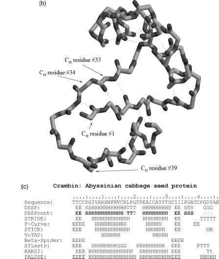
The regular secondary structures (helices and sheets), as defined by DSSP, comprise a bit more than half the protein residues (see Table 19.2), where the α-helix is most abundant with 31.3% followed by antiparallel β-sheets with 15.7% and parallel β-sheets with 5.7%. The remaining residues thus comprise a bit less than 50% (depending on the definition of regular structure used (see below)), which introduces a natural skewness of relevance within secondary structure prediction. The average lengths of the α-helix and p-sheet are 11.2 and 4.4 residues, respectively, which in terms of physical length interestingly enough are quite similar 16.8 and 14-15 Å, respectively (using physical distances for an α-helix of 1.5 Å per residue (Branden and Tooze, 1991) and residue span in fully extended strands is 3.2 Å residue in parallel β-sheets and 3.4 A per residue in antiparallel β-sheets (Creighton, 1993)).
TABLE 19.2. DSSP Secondary Structure Statistics from a Set of 707 Nonhomologous Protein Chains
a The following DSSP residues were counted: sheet H-bonded, middle and single bulge.
b The sum of the parallel and antiparallel sheet frequencies is higher than the total p-sheet residues, since a residue may be in two sheets of different type.
c The average length of sheets reported is different from the average length of connected “E” stretches (5.2 residues), since overlapping sheets are counted as one.
Residue Distributions for Secondary Structure
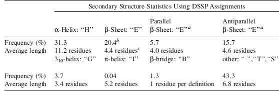
The amino acids typically found in a-helices differ considerably from those found in β-sheets (Figure 19.8). Alanine and leucine often occur in a-helices, while proline and glycine are rare. In p-sheets valine and isoleucine are over-represented, while glycine, aspartic acid and proline are under-represented. Shorter structures such as 310-helices and β-bridges have distinct residue distributions. For 310-helices, the alanine and leucine signal has disappeared, instead the sequences are dominated by proline which often is observed as a helix initiator and breaker. For β-bridges , we no longer find a preference for valine and isoleucine. This indicates the role of the side chain in defining secondary and tertiary structure. In general, these preferences have long been the basis of secondary structure prediction methods.
Comparison
The secondary structure assignment schemes delineated above have each been designed using one or more aspects of protein structure and with one or more applications in mind. Good quality assignments applied within CD spectroscopy analyses may not necessarily be optimal when applied within structure comparison or vice versa. It is therefore inherently difficult to perform a qualitative comparison among protein secondary structure assignments, so the main focus of the comparison presented will be quantitative. In essence one should choose the secondary structure assignment scheme that is most consistent with the investigation where it is applied.
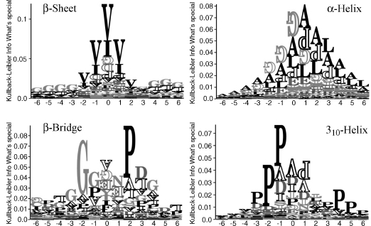
We used the simple structure of Crambin as an example to point out differences in the assignment schemes (Figure 19.9, note that the P-Curve assignment was taken from the original publication, Sklenar et al., 1989). When comparing the three-class assignments (a-helix, β-sheet, and other), STRIDE and DSSP are identical except for one residue at the C-cap of an a-helix, whose last H-bond is weak as reported by DSSPcont (reported in the figure as a grey letter). This assignment was confirmed by XTLsstr and KAKSI with some variation on cap assignments. P-Curve, STICK and PALSSE also assigned the same elements with capping variations, but reported an additional helix or sheet towards the protein’s C-term. Looking at the sheet region in detail (Figure 19.9b), we see that the residues 39 and 40, assigned sheet by P-Curve only, are distant from any residue on a putatively pairing strand. According to Pauling, such an assignment would not be valid. The two sheets have been extended by beta-spider showing that high backbone-backbone packing energy not caught by standard H-bonds is keeping the strands together. Longer sheets were also identified by XTLsstr, KAKSI, PALSSE and partially by STICK and P-Curve indicating that the backbone conformation is extended also for these amino acids, so the extension of the two DSSP/STRIDE sheets appears reasonable. VoTAP identifies the two primary α-helices, but is the only method which, for this particular protein, does not assign the two sheets observed by other methods.
Figure 19.8. Sequence distributions for secondary structure. The four graphs show alignment statistics for β-sheets, α-helices, β-bridges and 310-helices, by the Kullback–Leibler information at positions surrounding the one assigned (position 0). The number of aligned segments are: (a-helix) 41803, (310-helix) 4952, (β-sheets) 27320, (β-bridges) 1851. These segments were retrieved from a data set of 707 nonhomologous protein chains using the DSSP assignment. At a given position, we therefore observed the 20 amino acids with a certain frequency; the Kullback–Leibler information calculates the information content of the observed frequencies with respect to the background frequencies (irrespectively of the structure). The more an observed set of frequencies differs from the background, the higher the respective letter. If an amino acid at a given position is observed less frequently than in the background, it is drawn upside-down and hollow.
Are the discrepancies observed for Crambin representative? Secondary structure capping assignment do indeed constitute the major differences between methods as the exact specification of where a regular secondary structure ends is not well defined as reported by Colloc’h et al. (1993) for DSSP, P-Curve, and DEFINE. Investigating DSSP in particular, we also found variability of where the helix or sheet starts and ends between high-quality NMR models for the same protein, where the NMR model variability was found to correlate with inherent protein motion (Andersen et al., 2002). Helix and sheet core segments are also the assignments which correlate best with circular dichroism spectra (Sreerama et al., 1999).
Martin et al. (2005) have performed a comparison of some of the methods described above on a high-quality X-ray dataset (resolution < 1.7Å and R-factor < 0.19) containing 689 protein structures. They used a comparison score called C3 which compares two assignments as the number of identical regular secondary structure residue assignments relative to the total number of residues assigned to a regular structure, where the helix and sheet class assignments were compared. They found that DSSP and STRIDE are very similar (C3 = 95%) followed by the expert assignments in PDB (C3 > 87%). KAKSI is then the nearest neighbor to the group with C3 in the 81-84% range followed by PSEA and XTLsstr in the 78-81% range. XTLsstr differs the most from the other assignment methods with a C3 score down to 76% when compared to PSEA. Similar to what Colloc’h et al. (1993) has reported for DSSP; Martin et al. (2005) found that STRIDE assigns many short helices.
Another observation from the Crambin example is that the methods do not mix helix and sheet assignments on the same residue. This has generally been observed to hold true for DSSP, P-Curve, and DEFINE, where only 0.32% of the residues showed conflicts between helix and sheet assignments (Colloc’h et al., 1993).
Figure 19.9. Protein secondary structure for Crambin. The structure of the small protein Crambin (Teeter, 1984, PDB: 1CRN) is shown from two angles: (a) the image of the two helices and (b) the central short sheet. (c) The overall assignment of secondary structure is shown for the different assignment methods, where the overall elements were found to agree between most methods shown. Please note that beta-spider only assigns sheets and the DSSPcont assignments have been discretized to crisp (100%: bold or space), high ( > 90%: normal), mixt ( > 50%: grey) variants of the DSSP assignment. Each assignment method was used with its default/standard settings supplied.

APPLICATIONS OF SECONDARY STRUCTURE
Secondary structure is being used in many areas of structural bioinformatics, from structure visualization, classification, and comparison to predictions, all covered in this book. Here we will delineate some areas where secondary structure is applied in investigations within different contexts, for example, in understanding biological processes and disease.
Secondary Structure and Protein Function
Circular dichroism spectroscopy is often used to measure differences in protein secondary structure contents under different conditions such as mutated residues or changing environments. An example is the thimet met allo endo-peptidase (THOP1) which is known to be modulated by changes in calcium concentration. To study how this change comes about, key aspartic acid residues believed to bind calcium have been mutated, and the calcium induced change in a-helix content studied by CD (Oliviera, 2005). See also Chapter 21 describing functional inference from structure.
Secondary Structure and Disease
Protein aggregation plays an important part in several well-known diseases such as Alzheimer’s, Parkinson’s, Huntington’s, and prion disease (Kajava et al., 2006). The internal structure of amyloid fibrils in Alzheimer’s disease (AD) and type 2 diabetes is a ladder of β-sheet structure arranged in a cross-β conformation (Stromer and Serpell, 2005). Whether, for example, the amyloid-β plaques are causing Alzheimer’s disease or are mere agglomerates of excess amyloid-β is debated (Watson et al., 2005), but antiaggregates breaking the β-sheet formation are investigated to prevent AD (Chacon et al., 2004; Rzepecki et al., 2004). The formation of amyloid aggregation has been studied in close detail by Cerda-Costa et al. (2007), who found that the C-terminus of the molecule (comprising the last and edge β-strand ) is the major contributor to amyloid fibril formation. 3D structure analysis revealed the stability of amyloid fibrils, their self-seeding characteristic and their tendency to form polymorphic structures (Nelson et al., 2005).
A conserved N-capping box has been found to be important for the structural autonomy of the prion α-helix, where the disease associated D202N mutation destabilizes the helical conformation (Gallo et al., 2005).
Secondary Structure Mimicking Compounds
To develop a drug that can inhibit protein-protein interactions, compounds are being specifically synthesized to mimic helices and strands (Song et al., 2001; Kutzki et al., 2002; Antuch et al., 2006). Antuch et al. reported a-helix mimetic compounds disrupting the Bcl-w/Bak protein-protein interaction, which is important in cancer (Wagner, 2005). Song et al. described nonpeptidic β-strand mimetic compounds that inhibit the HIV-1 protease dimer-ization necessary for its enzymatic activity. Helices represent one of the most common recognition motifs in proteins (Che et al., 2007), therefore characterization and analysis of the secondary structures involved in protein-protein interactions becomes important. See also Chapter 27 for a description of protein-ligand design.
Secondary Structure and Alignment
Taking local structural characteristics into account improves the detection of remote homologues and the alignment quality (Wallqvist et al., 2000; Shi et al., 2001; Qiu and Elber, 2006). In FUGUE, Shi et al. took the secondary structure, solvent accessibility, and hydrogen bonding status into account when aligning structures and sequences, where the alignment gap penalties are dependent on secondary structure and its conservation. SSALN, a similar method by Qiu and Elber (2006), was found to outperform CLUSTALW and GenThreader using the Fisher’s benchmark.
Secondary Structure Capping
Helix capping has recently been studied in greater detail, for example, the capping dynamics of a glycine αL C-capping motif has been studied in detail (Bang et al., 2006). Bang et al., using chemical synthesis, X-ray crystallography, and thermodynamic data, determined that local conformational strain is responsible for most of the energy penalty in an αL C-capping motif (Rose, 2006). Helix caps are often stabilized by H-bonds other than the ones used for assignment (described above), as shown by Manikandan and Ramakumar (2004) for the C—H .. H-bond. The donor carbon studied was Cα,Cβ,Cγ,Cδ or Cε, depending on the residue, and the acceptor was the backbone C’=O oxygen. The α-helices were assigned using PROMOTIF (Hutchinson and Thornton, 1996) and their ends defined using the Aurora-Rose nomenclature (Aurora and Rose, 1998) with N-terminal residues as N-cap to N5 and C-terminal residues as C5 to C’’’. They found on average 1.5 and 3.9 C—H... OH-bonds per N- and C-term, respectively, thus indicating their relevance in stabilizing α-helix caps.
CONCLUSION
Assigning secondary structure from 3D coordinates is an important problem. Many successful solutions have been proposed over the past 25 years. One of the first automated assignment schemes was DSSP, which has become the standard in the field, followed by STRIDE. In fact, secondary structure assignment may be one of the exceptional examples of tools in structural biology and bioinformatics that have not been revolutionized by the explosion of data. For most residues, most of the available methods agree in their assignment. Methods tend to differ mainly in locating the caps of regular secondary structure segments and in distinguishing among more subtle differences (e.g. α-, 310-, or π-helix). These differences reflect the aspects used for the assignment and the application(s) for which the method was designed. Furthermore, there are indications that some fuzziness in the caps is inherent to protein motion (observed by NMR and CD) and that structural homologues also tend to differ more frequently there. Since the applications of secondary structure vary, their assignment schemes will as well, due to the differences in objectives. Optimization for structure comparison will aim at a high-regular structure content, while optimization for prediction will aim at clear capping signals and optimization for spectroscopists will aim at reflecting the experimental readout, so the story will continue.
ABBREVIATIONS
| 3D | three-dimensional |
| CD | circular dichroism |
| DEFINE | method assigning secondary structure from 3D coordinates based on linear distance masks of ideal secondary structure (Richards and Kundrot, 1988) |
| DSSP | program and database assigning secondary structure and solvent accessibility for proteins of known 3D structure from hydrogen bonding patterns |
| DSSPcont | continuous assignment of secondary structure for proteins of known 3D structure (Andersen et al., 2002) |
| H-bond | hydrogen bond |
| NMR | nuclear magnetic resonance |
| P-Curve | curvature-based assignment of secondary structure from 3D (Sklenar et al., 1989) |
| PDB | Protein Data Bank of experimentally determined 3D structures of proteins (Berman et al., 2000) |
| RMSD | root-mean square deviation |
| STRIDE | secondary STRuctural IDEntification method to assign secondary structure from 3D using hydrogen bonds and torsion angles (Frishman and Argos, 1995) |
| VoTAP | Voronoï tessellation based protein secondary structure assignment (Dupuis et al., 2004) |
ACKNOWLEDGMENTS
Thanks to Jinfeng Liu (CUBIC, Columbia) for computer assistance and Jenny Gu for helpful comments on the manuscript. The work of BR was supported by grants 1-P50-GM62413-01 and RO1-GM63029-01 from the National Institutes of Health. Last, not the least, thanks to all those who deposit their experimental data in public databases, and to those who maintain these databases.