2
FUNDAMENTALS OF PROTEIN STRUCTURE
THE IMPORTANCE OF PROTEIN STRUCTURE
Most of the essential structures and functions of cells are mediated by proteins. These large, complex molecules exhibit a remarkable versatility that allows them to perform a myriad of activities that are fundamental to life. Indeed, no other type of biological macromolecule could possibly assume all of the functions that proteins have amassed over billions of years of evolution.
Any consideration of protein function must be grounded in an understanding of protein structure. A fundamental principle in all of protein science is that protein structure leads to protein function. The distinctive structures of proteins allow the placement of particular chemical groups in specific places in three-dimensional spaceThink of this like a 3D key-value store, where the "key" is the location in 3D space and the "value" is a specific chemical group. The precise positioning of these groups is what enables proteins to perform their functions.. It is this precision that allows proteins to act as catalysts (enzymes)Catalysts are molecules that speed up chemical reactions without being consumed themselves. In computer science terms, think of enzymes as highly optimized functions that transform input molecules into output molecules, but can be reused indefinitely. for an impressive variety of chemical reactions. Precise placement of chemical groups also allows proteins to play important structural, transport, and regulatory functions in organisms. Since protein structure leads to function and protein functions are diverse, it is no surprise that protein structure is similarly diverse. Further, the functional diversity of proteins is expanded through the interaction of proteins with small molecules, as well as other proteins.
For those who wish to study protein structure, this diversity represents a challenge. Upon their determination of the first three-dimensional globular protein structure (the oxygen-storage protein myoglobin) in 1958, John Kendrew and his coworkers registered their disappointment (Kendrew et al., 1958):
Perhaps the most remarkable features of the molecule are its complexity and its lack of symmetry. The arrangement seems to be almost totally lacking in the kind of regularities which one instinctively anticipates, and it is more complicated than has been predicated by any theory of protein structure.This is analogous to looking at compiled machine code for the first time - while we expect to find clear patterns and structure, the reality is often much more complex and seemingly chaotic. Just as we later discovered higher-level patterns in machine code, researchers later found important regularities in protein structure.
Despite these initial frustrations, subsequent studies of the myoglobin structure based on higher quality data (Kendrew, 1961) revealed that the protein did have some regularities; these regularities were also observed in other protein structures.
Decades of research has now yielded a coherent set of principles about the nature of protein structure and the way in which this structure is utilized to effect function. These principles have been organized into a four-tier hierarchy that facilitates description and understanding of proteins: primary, secondary, tertiary, and quaternary structure. This hierarchy does not seek to precisely describe the physical laws that produce protein structure but is rather an abstraction to make protein structural studies more tractable.
THE PRIMARY STRUCTURE OF PROTEINS: THE AMINO ACID SEQUENCE
Amino Acids
Proteins are linear polymers of amino acidsThink of amino acids as the "primitive data types" of biology. Just like how you can build complex data structures from primitive types, proteins are built by chaining together these basic building blocks.,1 and it is the distinct sequence of component amino acids that determines the ultimate three-dimensional structure of the protein. The sequence of a protein is often referred to as its primary structure. The concept of proteins as linear amino acid polymers was initially proposed by Fischer and Hofmeister in 1902This was a revolutionary idea at the time - imagine discovering that all software is ultimately just a sequence of 1s and 0s, when everyone thought programs were something completely different!. At that time, the prevailing theory in protein science was that proteins lacked a regular structure and consisted of loose associations of small molecules (colloids). This issue was hotly debated for over 20 years, until the linear polymer theory achieved general acceptance in the late 1920s (Fruton, 1972). In 1952, Fred Sanger made the important discovery that proteins could be distinguished by their amino acid sequences (Sanger, 1952). Indeed, he found that proteins of exactly the same type have identical sequences. Sanger's work helped to remove remaining doubts about the accuracy of the linear polymer theory.
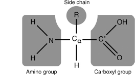
Amino acids are small molecules that contain an amino group (NH2), a carboxyl group (COOH), and a hydrogen atom attached to a central alpha (α) carbonThink of this as the common "interface" that all amino acids implement. Just like how different classes in object-oriented programming share common methods but have different implementations, all amino acids share this basic structure but differ in their side chains.. In addition, amino acids also have a side chain (or R group) attached to the α-carbon. It is this group, and only this group, that distinguishes one amino acid from another. Furthermore, the side chain confers the specific chemical properties of the amino acid.
Figure 2.1. The structure of a prototypical amino acid. The chemical groups bound to the central alpha (α) carbon are highlighted in gray. The R-group represents any of the possible 20 amino acid side chains.
Cellular genomes contain coded instructions for the production of multiple proteins, and there are 20 amino acids that can be incorporated into a protein via these instructions. The resulting sequence of a protein can contain any combination and number of the 20 amino acids, in any order. Though amino acids had been known to be the building blocks of proteins prior to the turn of this century, the exact set of amino acids used in proteins was not determined until 1940This is analogous to the development of character encoding standards - while we knew text was made up of characters, it took time to standardize on ASCII/Unicode. Similarly, it took time to discover the standard "character set" of life.. This set of 20 amino acids is considered "standard" in that it is common to all observed organisms. Modified forms of these 20 amino acids do exist in proteins, but these are the product of modifications that occur subsequent to protein synthesis.
There are two recent additions to the 20 standard amino acids that, although they are infrequently observed, merit discussion. In a few proteins, a selenium-containing residue, selenocysteine (Sec), can be incorporated duringprotein synthesis (Zinoni et al., 1986; Atkins and Gesteland, 2000), and the lysine derivative, pyrrolysine (Pyl), has been found in some proteins in methanogenic bacteria (Srinivasan, James, and Kryzycki, 2002). Both of these amino acids are encoded by a signal that normally serves to stop synthesis of the protein chain. However, if the necessary cellular machinery is available to incorporate these amino acids, the stop signals are co-opted for insertion of what are termed the 21st and 22nd amino acids.
Interestingly, the cellular machinery that incorporates amino acids into a protein chain can be extrinsically altered to incorporate amino acids not included in the standard set (Wang, 2001; Wang, Xie, Schultz, 2006). This allows researchers to genetically encode unnatural amino acids that can fluoresce, are glycosylated, can bind metal ions, or are redox-active, into both prokaryotic and eukaryotic organisms. Incorporation of these amino acids serves as an experimental tool for researching aspects of protein structure. To date, over 30 unnatural amino acids have been successfully encoded using this method.
The 20 standard amino acids can be loosely grouped into classes based on the chemical properties conferred by their side chains. Three classes are commonly accepted: hydrophobic, polar, and charged. Within these classes, additional subclassifications are possible, for example, aromatic or aliphatic, large or small, and so on (Taylor, 1986). Figure 2.2 provides one possible amino acid classification.
A few amino acids have distinctive properties that merit closer attention. The side chain of proline forms a bond with its own amino group, causing it to become cyclic.2 Though proline generally exhibits the properties of an aliphatic nonpolar amino acid, the cyclic construction limits its flexibility, and this impacts the overall structure of proteins that contain it.
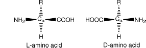
Glycine is also of interest because its side chain consists only of a single hydrogen atom. In effect, glycine has no side chain, and this confers a unique property on it amongst the 20 amino acids: glycine is achiral. Any carbon bound to four distinct groups (as seen in the other 20 amino acids) is said to be chiral (Figure 2.3). Chiral molecules can exist in two distinct forms, which are in effect mirror images of each other. These two forms have been deemed the d and l forms.3 In 1952, Fred Sanger discovered that proteins seem to be constructed entirely of l-amino acids (Sanger, 1952). Indeed, for unknown reasons, all known organisms have standardized upon the l form of amino acids for the genetically directed production of proteins. d-Amino acids are seen in polypeptides in rare cases, but they are a result of direct enzymatic synthesis (Kreil, 1997).
Figure 2.2. The 20 "standard" amino acids used in proteins, grouped on the basis of the properties of their side chains. The shared amino acid structure is shaded gray. Each amino acid is labeled with its full name, followed by its three-letter and one-letter abbreviations. This classification groups amino acids on the basis of the form that predominates at physiological conditions (note that their amino and carboxyl groups are charged under these conditions). Although this classification is a useful guideline, it does not convey the full complexity of side chain properties. For example, tryptophan and histidine do not fall clearly into a single grouping. Tryptophan is somewhat polar due to the nitrogen in its five-membered ring but has a hydrophobic six-membered ring at the end of its side chain. Histidine can be neutral polar and/or positively charged under physiological conditions.
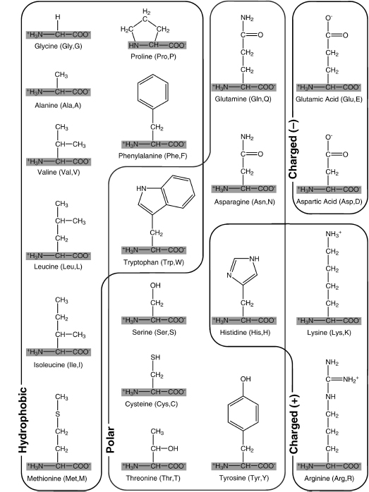
Figure 2.3. The possible stereoisomers of a prototypical amino acid. Note that these structures are mirror images of each other. The L-form is the only type incorporated into proteins via the genetic machinery.
The Peptide Bond
Amino acids can form bonds with each other through a reaction of their respective carboxyl and amino groups. The resulting bond is called the peptide bond, and two or more amino acids linked by such a bond are referred to as a peptide (Figure 2.4). A protein is synthesized by the formation of a linear succession of peptide bonds between many amino acids (as directed by the genetic code) and can thus be referred to as a polypeptide. Once an amino acid is incorporated into a peptide, it is referred to as an amino acid residue, and the atoms involved in the peptide bond are referred to as the peptide backbone.
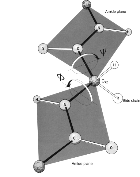
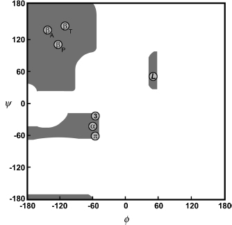
The specific characteristics of the peptide bond have important implications for the three-dimensional structures that can be formed by polypeptides. The peptide bond is planar and quite rigid. Therefore, the polypeptide chain has only a rotational freedom about the bonds formed by the α-carbons. These bonds have been termed the Phi (Φ) and Psi (ψ) angles (Figure 2.5). However, rotational freedom about the Φ (Cα—N) and ψ (Cα—C) angles is limited by steric hindrance between the side chains of the residues and the peptide backbone. Consequently, the possible conformations of a given polypeptide chain are quite limited. A Ramachandran plot (a plot of Φ versus ψ angles) maps the entire conformational space of a polypeptide and illuminates the allowed and disallowed conformations (Ramachandran and Sasisekharan, 1968) (Figure 2.6). These plots were developed by G.N. Ramachandran in the late 1960s based on studies of sterically allowed Φ and ψ angle combinations. See Chapter 14 for a more detailed discussion of these plots.
Some key exceptions to these conformational limitations can be attributed to glycine and proline. As noted previously, the side chain of glycine (a single hydrogen atom) is very small. There is markedly reduced steric hindrance about the Φ and ψ angles of this residue, thus expanding the possible conformational space. Conversely, the cyclic bond present in proline residues reduces the conformational freedom beyond the limitations observed with other amino acids.
Figure 2.4. The peptide bond. Two peptide units (amino acid residues) are shown shaded in light gray. The peptide bond between them is shaded in dark gray. The R-group represents any of the possible 20 amino acid side chains.

Figure 2.5. The planar characteristics of the peptide bond, and rotation of the peptide backbone about the Cα atom. Note the two planar peptide bonds about a central alpha carbon, shown here as a ball-and-stick model. Rotation is only possible about the Φ (Cα_N) and ψ (Cα_C') angles. Arrows about the two angles show the direction that is considered positive rotation. In this figure, both angles are approximately 180°. From R.E. Dickerson and I. Geis. The Structure and Action of Proteins. New York: Harper & Row, 1969.
THE SECONDARY STRUCTURE OF PROTEINS: THE LOCAL THREE-DIMENSIONAL STRUCTURE
The secondary structure of a protein can be thought of as the local conformation of the polypeptide chain, independent of the rest of the protein. The limitations imposed upon the primary structure of a protein by the peptide bond and hydrogen bonding considerations dictate the secondary structure that is possible. During the course of protein structure research, two types of secondary structure have emerged as the dominant local conformations of polypeptide chains: alpha (α) helix and beta (β) sheets. Interestingly, these structures were actually predicted by Linus Pauling, Robert Corey, and H.R. Branson, based on the known physical limitations of polypeptide chains, prior to the experimental determination of protein structures (Pauling and Corey, 1951a; Pauling, Corey, and Branson, 1951). Indeed, if the Ramachandran plot is examined, helices and sheets contain Φ and ψ angles that fall within the two largest regions of allowed conformation (Figure 2.6). These structures exhibit a high degree of regularity: the particular Φ and ψ angle combinations in the polypeptide chain are approximately repeated for the duration of the secondary structure.
Figure 2.6. A schematic representation of a Ramachandran plot (a plot of Φ versus ψ angles). Gray regions denote the allowed conformations of the polypeptide backbone. Circles indicate the paired angle values of the repetitive secondary structures. Definitions of symbols: βA, antiparallel β–sheet; βP, parallel β–sheet; βT, twisted β–sheet (parallel or antiparallel); α, right-handed α-helix; L, left-handed helix; 3, 310 helix; π, π helix.
Although helices and sheets satisfy the peptide bond constraints, this is not the only factor that explains their ubiquity. Both of these structural elements are stabilized by hydrogen bond interactions between the backbone atoms of the participating residues, making them a highly favorable conformation for the polypeptide chain. Helices and sheets are the only regular secondary structural elements present in proteins. However, irregular secondary structural elements are also observed in proteins and are vital to both structure and function.
α-Helices
A helix is created by a curving of the polypeptide backbone such that a regular coil shape is produced. Because the polypeptide backbone can be coiled in two directions (left or right), helices exhibit handedness. A helix with a rightward coil is known as a right-handed helix. Almost all helices observed in proteins are right-handed, as steric restrictions limit the ability of left-handed helices to form. Among the right-handed helices, the α helix is by far the most prevalent.
An α-helix is distinguished by having a period of 3.6 residues per turn of the backbone coil. The structure of this helix is stabilized by hydrogen bonding interactions between the carbonyl oxygen of each residue and the amide proton of the residue four positions ahead in the helix (Figure 2.7). Consequently, all possible backbone hydrogen bonds are satisfied within the α-helix, with the exception of a few at each end of the helix, where a partner is not available.
Figure 2.7. Diagram of an α-helix using a ball-and-stick model. The bonds forming the backbone of the polypeptide are shaded dark. The α-helix is stabilized by internal hydrogen bonds formed between the carbonyl oxygen of each residue and the amide proton of the residue four positions ahead in the helix, shown here as dashed lines. Note that the polypeptide backbone curves toward the right, and as such the α-helix is a right-handed helix. From R.E. Dickerson and I. Geis. The Structure and Action of Proteins. New York: Harper & Row, 1969.
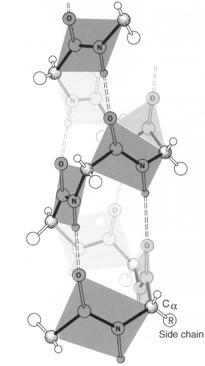
Figure 2.8. The hydrogen bonding patterns of different helical secondary structures. The peptide backbone is shown in an extended conformation, with an arrow denoting the hydrogen bonding pairings that would occur in each type of helix. The common α-helix, depicted in Figure 2.7, forms hydrogen bonds between the carbonyl oxygen of each residue and the amide proton of the residue four positions ahead in the helix. The 310 helix forms hydrogen bonds between the carbonyl oxygen of each residue and the amide proton of the residue three positions ahead, forming a more narrow and elongated helix. The π-helix forms hydrogen bonds between the carbonyl oxygen of each residue and the amide proton of the residue five positions ahead, forming a wider helix. The 27 ribbon is not a regular secondary structure, but is shown here to demonstrate all possible hydrogen bond pairings. From R.E. Dickerson and I. Geis. The Structure and Action of Proteins. New York: Harper & Row, 1969.
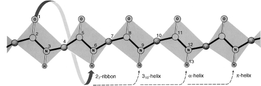
Other helices have also been observed in proteins, though much less frequently due to their less favorable geometry. The 310 helix has a period of three residues per turn, with hydrogen bonds between each residue and the residue three positions ahead (Taylor, 1941; Huggins, 1943) (Figure 2.8). This type of helix is usually seen only in short segments, often at the ends of an α-helix. The very rare pi (π) helix has a period of 4.4 residues per turn, with hydrogen bonds between each residue and the residue five positions ahead, and has only been seen at the ends of α-helices (Low and Baybutt, 1952).
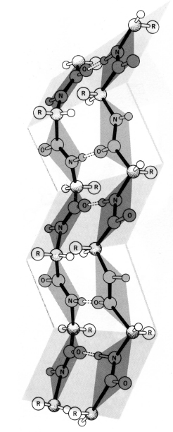
Unlike helices, β-sheets are formed by hydrogen bonds between adjacent polypeptide chains rather than within a single chain. Sections of the polypeptide chain participating in the sheet are known as β-strands. β-strands represent an extended conformation of the polypeptide chain, where Φ and ψ angles are rotated approximately 180° with respect to each other. This arrangement produces a sheet that is pleated, with the residue side chains alternating positions on opposite sides of the sheet (Figure 2.9).
Two configurations of β-sheet are possible: parallel and antiparallel. In parallel sheets, the strands are arranged in the same direction with respect to their amino terminal (N) and carboxy terminal (C) ends. In antiparallel sheets, the strands alternate their amino and carboxy terminal ends, such that a given strand interacts with strands in the opposite orientation. β-sheets can also form in a mixed configuration, with both parallel and antiparallel sections, but this configuration is less common than the uniform types mentioned above. Almost all β-sheets exhibit some degree of twist when the sheet is viewed edge on, along an axis perpendicular to the direction of the polypeptide chains. This twist is generally right-handed.
Figure 2.9. Diagram of an antiparallel β-sheet using a ball-and-stick model. The bonds forming the backbone of the polypeptide are shaded dark. The β-sheet is stabilized by hydrogen bonds shown here as dashed lines) formed between the carbonyl oxygen of a residue on one strand and the amide proton of a residue on the adjacent strand. Note that this arrangement produces a sheet that is pleated, with the residue side chains alternating positions on opposite sides of the sheet. From R.E. Dickerson and I. Geis. Hemoglobin: Structure, Function, Evolution, and Pathology. Menlo Park, CA: The Benjamin/Cummings Publishing Company, 1983.
In order for β-strands to interact with each and form a sheet, the amino acid backbone must form a turn. The simplest and tightest turn is the β-hairpin turn (also called type I and type II turns, depending on the conformation of the backbone). Other stereochemically allowed turns include the mirror images of the type I and type II turns (denoted type I' and type II') as well as type III and type VI turns (Rotondi, 2006). All are observed in naturally occurring proteins and the type I turn appears to be most commonly used, frequently occurring between antiparallel strands.
An important variant of the classical β-sheet structure is the β-bulge. The β-bulge, most often observed in antiparallel β-sheets, is a hydrogen bond between two residues on one β-strand with one residue on the adjacent strand (Richardson, Getzoff, and Richardson, 1978; Chan et al., 1993). This structure can alter the direction of the polypeptide chain and augment the right-handed twist of the sheet (Richardson, 1981).
Other Secondary Structure
α-helices and β-sheets account for the majority of secondary structure seen in proteins. However, these regular structures are interspersed with regions of irregular structure that are referred to as loop or coil. Loop regions are usually present at the surface of the protein. These regions are often simply transitions between regular structures, but they can also possess structural significance and can be the location of the functional portion, or active site, of the protein.
Most of these structures were predicted and observed in the 1960s and 1970s (Venkatachalam, 1968; Chandrasekaran et al., 1973; Lewis et al., 1973; Chou and Fasman, 1977). Because of their irregularity, these elements are difficult to classify. However, some types of structures are ubiquitous enough to have been loosely categorized. β-Hairpin turns (described above) involve the minimum number of residues (4-5); transitions involving more residues (6-16) are often referred to as omega (Ω) loops because they resemble the shape of the capital Greek letter omega (Richardson, 1981). These loops can involve complex interactions that include the side chains, in addition to the polypeptide backbone. Extended loop regions involving more than 16 residues have also been observed.
Although loop regions are irregular, these structures are generally as well ordered as the regular secondary structures. However, experimental determination of protein structures has shown that some loop regions are disordered and thus do not achieve a stable structure. This type of loop region is referred to as random coil.
THE TERTIARY STRUCTURE OF PROTEINS: THE GLOBAL THREE-DIMENSIONAL STRUCTURE
The tertiary structure of a protein is defined as the global three-dimensional structure of its polypeptide chain. In a striking display of foresight, Alfred Mirsky and Linus Pauling correctly described several important aspects of tertiary structure in 1936 when they presented the following hypothesis on the nature of proteins (Mirsky and Pauling, 1936):
... one polypeptide chain which continues without interruption throughout the molecule ... folded into a uniquely defined configuration, in which it is held by hydrogen bonds between the peptide nitrogen and oxygen atoms and also between the free amino and carboxyl groups of the diamino and dicarboxyl amino acid residues.
The prediction of Mirsky and Pauling is especially striking considering that very little structural data were available and the linear polymer theory was still unproven at that time. As described previously, hydrogen bonds are important in the stabilization of secondary structure, but Mirsky and Pauling correctly divined their importance in tertiary structure stabilization as well.
While Mirsky and Pauling correctly predicted the role of hydrogen bonds in protein structure, it subsequently became apparent that other forces would also be important. With the determination of the structure of myoglobin by John Kendrew (Kendrew et al., 1958), protein scientists at last could begin to confirm many of their assumptions about various aspects of tertiary structure. Subsequent determination of the myoglobin structure using more accurate data (Kendrew et al., 1960), and the determination of the structure of hemoglobin by Max Perutz (Perutz et al., 1960), allowed scientists to begin to directly catalog aspects of the tertiary structure protein for the first time. Years of experimentation has now made it possible to understand how secondary structural elements combine in three-dimensional space to yield the tertiary structure of a protein.
Side Chains and Tertiary Structure
There are a wide variety of ways in which the various helix, sheet, and loop elements can combine to produce a complete structure. These combinations are brought about largely through interactions between the side chains of the constituent amino acid residues of the protein. Thus, at the level of tertiary structure the side chains play a much more active role in creating the final structure. In contrast, backbone interactions are primarily responsible for the generation of secondary structure (particularly in the case of helices and sheets). Most proteins each have a distinctive tertiary structure; the secondary structural elements of these proteins will always form the same tertiary structure. This consistency is vital to proper function of the protein.
Protein Folding
The final three-dimensional tertiary structure of a protein is commonly referred to as its fold. Appropriately, the process by which a linear polypeptide chain achieves its distinctive fold is known as protein folding. Protein folding is a complex process that is not yet completely understood, but many of the important principles are known. In a series of experiments in the early 1960s, Christian Anfinsen and his colleagues demonstrated that a small protein (ribonuclease) could be completely unfolded with chemicals, but when the protein was placed back into normal physiological conditions, it would spontaneously refold and regain full activityThis is like discovering that a compiled program, when scrambled into random bytes, could spontaneously reassemble itself into the correct sequence when placed in the right environment. It showed that the "compilation" from sequence to structure is deterministic and reversible., as if it had never been unfolded in the first place (Anfinsen et al., 1961; Haber and Anfinsen, 1962). Anfinsen's work demonstrated a key concept in protein folding: the primary structure of the protein contains all of the information required for it to acquire the correct fold. In other words, proteins are capable of self-assembly. Anfinsen also proposed that the native fold of a protein corresponded to its lowest potential energy state and that protein folding was thus a process by which a protein chain spontaneously "falls" from the higher energy unfolded state to the lower energy folded state. Though this description of folding explained why proteins fold, it did not describe exactly how the process takes place.
Cyrus Levinthal demonstrated the remaining difficulties in protein folding with a simple thought experiment that measured the time a protein chain would take to find its lowest energy conformation through exhaustive search of all possible conformationsThis is similar to the traveling salesman problem in computer science - the number of possible paths grows factorially with the number of cities (or in this case, amino acids). Just like how we need better algorithms than brute force for TSP, proteins must use a more efficient folding strategy.. He reported that the universe would likely come to an end before the protein would fold!4 However, most proteins are known to fold in fractions of a second. This conflict between theory and experiment became known as Levinthal's paradox, demonstrating that the search for a protein's native state must not be random, but rather directed in some way such that the protein can fold rapidly.
The need for directed folding led to the current leading model for protein folding, initially proposed by Peter Wolynes and colleagues, in which the folding "energy landscape" is funnel-shapedThink of this like a cost/fitness function in optimization algorithms. Instead of randomly searching the space of possible configurations, the protein follows the gradient of the energy landscape, similar to how gradient descent algorithms work in machine learning. (Frauenfelder, Sligar, and Wolynes, 1991). The edges of the funnel correspond to high potential energy unfolded states, and as the protein folds it is directed down the funnel into lower energy states until it reaches its native fold. The difficulty with this model is how the protein chain avoids getting stuck in "dips" in the funnel that are low energy, but not the native (lowest energy) fold. The answer appears to be found in the evolutionary process itself. It appears the protein sequences have evolved not only to form their native structures but also to have smooth energy landscapes that lack significant dips. Indeed, small naturally evolved proteins have been observed to fold in a highly "cooperative" fashion. That is, the whole protein chain participates in the folding process, and once the protein begins to fold the transition from unfolded to folded state is extremely rapid, and discrete intermediate structures cannot be isolated. This cooperative folding capability appears to be a specific quality shared by natural sequences and is not necessarily seen in proteins that have been designed in the laboratoryThis is similar to how human-written code often contains edge cases and bugs, while evolved biological systems have been optimized through millions of years of testing to be robust and efficient.. Further, it should be noted that random polypeptide sequences will almost never fold into an ordered structure; an important property of natural protein sequences is that they have been selected by the evolutionary process to achieve a reproducible, stable structure (Richardson, 1992).
Larger proteins (> 100 residues) appear to fold based on the same principles, but their complexity leads to slower folding, often with clear transition states on the way to the native state, and a more modular folding pattern (Vendruscolo et al., 2003). For these proteins, the more complex folding landscape introduces a new risk: the partly folded protein could start to interact improperly with other proteins, leading to the formation of harmful protein aggregates (Dobson, 2003). To deal with this challenge, cells employ "molecular chaperones," which are proteins that help other proteins to fold correctly and avoid aggregation (Hartl and Hayer-Hartl, 2002).
Thus, protein sequences are subject to several disparate evolutionary pressures. They must fold smoothly, avoiding incorrect alternate structures on the way to the correct one, resist the formation of aggregates, and finally, form a stable native structure once folding is complete. The sequences of natural proteins encode all of these characteristics, allowing them to fold reliably. However, despite the deterministic nature of protein folding, it is not yet possible to accurately predict the final structure of a protein given only its sequence (see Section VII for a discussion of the methods currently used to tackle this problem).
Domains and Motifs
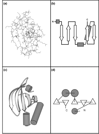
Within the overall protein fold, distinct domains and motifs can be recognized. Domains are compact sections of the protein that represent structurally (and usually functionally) independent regions. In other words, a domain is a subsection of the protein that would maintain its characteristic structure, even if separated from the overall protein. Motifs (also referred to as supersecondary structure) are small substructures that are not necessarily structurally independent; generally, they consist of only a few secondary structural elements. Specific motifs are seen repeatedly in many different protein structures; they are integral elements of protein folds. Further, motifs often have a functional significance and in these cases represent a minimal functional unit within a protein. Several motifs can combine to form specific domains. Please see Figure 2.10 for a brief history of protein structure representation and visualization of these domains and motifs.
Figure 2.10.
Schematic diagrams. One of the earliest pioneers in protein visualization was Irving Geis (Kendrew
et al., 1961; Dickerson and Geis, 1969), who created some of the most definitive representations of
protein structure. His hand-drawn depictions were so enlightening that they appear in textbooks to
this day (and appear in this chapter). While hand drawings are extremely valuable, they are
ultimately impractical because of the large number of protein structures that must be depicted (and
the unusual level of talent required). Arthur Lesk and Karl Hardman were the first to popularize the
use of computers to automatically generate schematic diagrams, given the (experimentally determined)
spatial coordinates of the atoms in the protein (Lesk and Hardman, 1982). For more on molecular
visualization, see Chapter 9.
The N-terminal domain of
the catalytic core of eukaryotic protein kinase A (PKA, PDB id 1APM: residues 35-123) is depicted
here using four different representations. This section of PKA contains a five-stranded antiparallel
β-sheet and three helices. Figure 2.10a depicts this
domain using an all-atom line representation. As can be seen, it is difficult to determine the
overall structural characteristics of this protein using such a representation. Because proteins are
often large and complex structures, views at the atomic level tend to obfuscatethe important
features. For this reason, a variety of schematic diagrams have been developed for the visual
representation of protein structure. These diagrams replace the individual residues with shapes that
represent the secondary structure they belong to and facilitate recognition of motifs and
domains.
Simple topology diagrams are two-dimensional
projections of the protein structure that are particularly useful for comparing the tertiary
structures of different proteins (Holbrook et al., 1970). In these diagrams, β-strands are
represented by arrows that point from the N-terminus to the C-terminus; α-helices are represented by
cylinders. Connections between the secondary structural elements (loops) are simply represented as lines. These diagrams
clearly illustrate the topology (connectivity) between the secondary structural elements and
parallel or antiparallel nature of β-sheets (Figure
2.10b).
Cartoon diagrams illustrate the
topology of the protein, as well as the spatial relationship between the structural components.
These diagrams represent the three-dimensional structure of the protein as it actually occurs, with
the atoms replaced by the same elements used in topology diagrams. Initially conceived of by Jane
Richardson, and presented as hand drawings (Richardson, 1981), this representation is now very
commonly used in protein visualization software packages (Figure 2.10c). Figure 2.10a and c
was generated with the MolScript package (Kraulis, 1991), and is shown in an identical spatial
orientation. The cartoon images in Tables 2.1 and 2.2 were also generated with the MolScript package.
TOPS diagrams, developed by Michael Sternberg and
Janet Thornton, allow both the topology and the interaction of structural elements to be represented
in a two-dimensional format (Sternberg and Thornton, 1977). Here, the secondary structural elements
are viewed edge-on, as if they were projecting outward in a direction perpendicular to the plane of
the page. β-strands are represented by triangles; an upward-pointing triangle portrays a strand
pointing out of the page while a downward-pointing triangle portrays a strand pointing into the
page. Helices are represented by circles. Lines represent the loopsconnectingthese elements and also
help portray chain direction (Figure 2.10d). Software
is available to automatically generate these figures (Flores, Moss, and Thornton, 1994).
Molecular Interactions in Tertiary Structure
As with secondary structure, intramolecular forces are integral to defining and stabilizing the tertiary structure. The molecular interactions between structural elements, and individual side chains within these elements, help determine the protein fold. Because of the variety of chemical characteristics of the 20 standard amino acids, many types of interactions between them are possible. Furthermore, it is important to note that many proteins exist in an aqueous environment; intermolecular interactions with water (solvent) must be considered in addition to interactions within the protein itself.
A dominant molecular interaction in the tertiary structure of proteins is the hydrophobic effect (Tanford, 1978). Residues with hydrophobic side chains are packed into the core of the protein, away from the solvent, while charged and polar residues form the surface of the protein and are able to interact with polar water molecules and solvated ions. Although residues with hydrophobic side chains fit naturally into the core of the protein, their polar polypeptide backbone does not. For the backbone to participate in the hydro-phobic core, its hydrogen bonding groups must be satisfied such that their polarity is, in effect, neutralized. Ordered secondary structural elements (helices and sheets) provide this neutralization through their regular hydrogen bonding patterns. Thus, secondary structural elements are critical to the formation of the hydrophobic core.
Residues with polar side chains can also participate in the hydrophobic core. They are, however, subject to same restrictions as the polypeptide backbone: they must be involved in an interaction that neutralizes their polarity. Buried polar residues can form hydrogen bonds with other polar residues, or with sections of the polypeptide backbone not participating in a regular secondary structure. Alternately, in some proteins small pockets exist in which buried polar residues satisfy their hydrogen bonds with water molecules. These water molecules are completely isolated from the solvent and are integral to the protein structure.
Charged residues can also occur within the hydrophobic core. This arrangement is possible only if the charged residue is paired with another residue of opposite charge such that the net charge is zero. This interaction, initially proposed by Henry Eyring and Allen Stearn in 1939, is known as an ion pair or salt bridge (Eyring and Stearn, 1939).
Eyring and Stearn also surmised that covalent connections between residue side chains were important in maintaining tertiary structure (Eyring and Stearn, 1939). Indeed, covalent interactions have been observed in some proteins. However, only one of the standard 20 amino acids is capable of participating in a covalent linkage: cysteine. The disulfide bond (—S—S—) can occur between the thiol (—SH) groups of two cysteine residues.5 This interaction exists in proteins to further stabilize the protein fold. Cysteine residues do not always participate in disulfide bonds; in proteins, the majority of these residues are not part of a disulfide linkage.
Protein Modifications
Even though amino acids have a wide variety of chemical characteristics, chemical modifications and interaction with nonpolypeptide molecules can further extend the capabilities of proteins. At the level of tertiary structure, it is important to note these phenomena, as they can be critical to both the structure and the function of proteins.
The chemical properties of the 20 standard amino acids can be extended through side chain modification. In some cases, such modification can be indispensable to the proper formation of tertiary structures. For example, the protein collagen contains a modified proline residue, hydroxyproline, which greatly stabilizes the protein fold (Pauling and Corey, 1951b). In other cases, residue modification has no effect on fold, but rather extends the functional repertoire of the protein.
Molecules, such as carbohydrates and lipids, can be attached to the protein via covalent bonds with specific residues. Carbohydrate modifications are often seen on proteins that function extracellularly and are known to play a role in intracellular protein localization. Lipid modifications can help anchor a protein in the cell membrane.
Proteins can also associate with small molecules or metal atoms (covalently or noncovalently) to diversify their functional and structural capabilities. Many enzymes employ such molecules as cofactors, which assist them in chemical catalysis (Karlin, 1993). Other proteins require these molecules or atoms for proper tertiary structure formation. For example, the zinc-finger motif, a structural motif important for the interaction of some proteins with DNA, cannot form without the covalent interaction of a zinc atom with specific cysteine, or cysteine and histidine, residues (Lee, 1989).
Fold Space and Protein Evolution
One might imagine that the ways in which secondary structures can be combined to form a complete protein fold are almost limitless. Indeed, the variety of protein folds and the chemical diversity of their residues lead to a wide array of functions. This universe of extant folds is often called "fold space." Interestingly, currently available protein structure data suggest that fold space is in fact quite limited, relative to the range of folds that would seem possible a priori. Early estimates suggested that there might be about 1000 unique protein folds (Chothia, 1992; Govindarajan, Recabarren, and Goldstein, 1999; Wolf, Grishin, and Koonin, 2000). However, this number is now being approached by the available protein structure data and it appears likely it will be surpassed (Andreeva et al., 2004). More recent estimates suggest that the total number of natural folds lies somewhere between 1,000 and 10,000 (Koonin, Wolf, and Karev, 2002; Grant, Lee, and Orengo, 2004). It is likely that two forces have played a role in the observed limitation of fold space: divergent evolution of protein function and convergent evolution of protein structure.
In the case of divergent evolution, the number of extant protein folds is limited because they are derived from a relatively small group of shared common ancestor proteins. These early ancestor proteins would have "discovered" a stable fold, which has then been duplicated and re-used by organisms for many other functions over the course of evolution. Presumably, modification of an existing fold is more likely to occur than the spontaneous generation of a novel fold. There is clear evidence that this sort of modification has occurred over and over; it is possible because the link between protein structure and function is not direct (Todd, Orengo, and Thornton, 2001). Though protein structure leads to protein function, similar protein structures will not always have similar functions. There are many cases where two proteins have similar sequences and structures but differ by a few key amino acid residues in an active site and hence have very different functions. Thus, it is important to consider a protein's overall tertiary structure as a guide to the function of that protein, rather than a definition of the function (see Chapter 21). This functional versatility suggests the possibility that many protein folds will never be seen because organisms have simply not required or developed them.
In the case of convergent evolution, the number ofextant folds is limited because certain folds are biophysically much more favored, and so have been created independently in multiple cases. Certain folds are clearly overrepresented in the set of proteins of known structure, even when efforts are made to reduce the representational bias inherent in the Protein Data Bank (PDB) (Berman et al., 2000; see Chapter 11). In some cases, there is no discernable sequence similarity between proteins of similar fold, suggesting that they have converged upon a similar structure independently and do not share a common ancestor (Holm and Sander, 1996). Further, some protein folding models have suggested that a small subset of folds will be biophysically favored over all others (Govindarajan and Goldstein, 1996; Li et al., 1996). Hence, it is possible that many folds will never be seen because they are not structurally favorable, and other more favorable folds can be adapted to the needed functions.
The divergent and convergent protein evolution scenarios are not mutually exclusive, and both appear to have had a part in limiting the range of folds in fold space. Even though fold space appears limited, it is still complex enough to make classification and comprehension of protein folds difficult (see Chapters 17 and 18).
Biochemical Classification of Folds
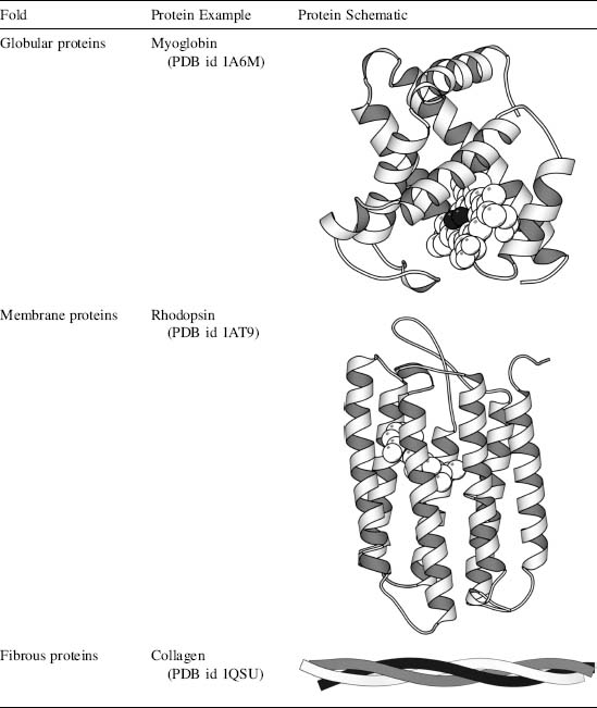
One method of protein classification partially sidesteps the issue of structural organization in favor of biochemical properties. Here, proteins are classified into three major groups: globular, membrane, and fibrous.
Globular proteins exist in an aqueous environment and thus fold as compact structures with hydrophobic cores and polar surfaces. They exhibit the "typical" structural elements that have been discussed above. This class of proteins is well represented in the PDB, partly because these structures are the easiest to determine experimentally (see Chapters 4-6). Because of the variety of determined structures available, globular proteins have been used as the basis for most protein structure studies (Berman et al., 2000). Indeed, the first two experimentally determined structures, myoglobin and hemoglobin, are globular (Kendrew et al., 1958; Perutz et al., 1958) (Table 2.1).
Membrane proteins exhibit many of the same characteristics as globular proteins, but they are distinguished in two important ways. First, they exist in an environment completely different from typical globular proteins: the cell membrane. In the interior of the cell membrane, the protein is surrounded by a hydrophobic environment. Thus, the regions of the protein within the cell membrane must have a hydrophobic surface in order to be stable. Some proteins exist almost entirely within the cell membrane, while others have membrane-spanning or membrane-interacting domains. Second, experimental structure determination (Chapters 4-6) of membrane proteins is more difficult than the determination of the structure of globular proteins. These proteins are very poorly represented in the PDB and thus are poorly understood. However, the structures that have been determined suggest that they use the same secondary structural elements and follow the same general folding principles as globular proteins (Table 2.1).
Fibrous proteins differ markedly from both membrane and globular proteins. These proteins are often constructed of repetitive amino acid sequences that form simple, elongated fibers. Their repetitive design is well suited to the structural roles they often play in organisms. Some fibrous proteins consist of a single type of regular secondary structure that is repeated over very long sequences. Others are formed from repetitive atypical secondary structures, or have no discernable secondary structure whatsoever (Table 2.1).
TABLE 2.1 Biochemical Folds
Structural Classification of Folds
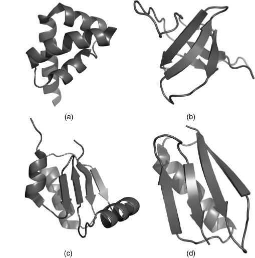
As more and more protein structures have been determined, development of increasingly specific fold classifications has become possible. Cyrus Chothia and Michael Levitt derived one of the first such classifications, which grouped proteins on the basis of their predominant secondary structural element (Levitt and Chothia, 1976). This classification consisted of four groups: all α, all β, α/β, and α + β (Figure 2.11). All α-proteins, as the name suggests, are based almost entirely on an α-helical structure, and all β-structures are based almost entirely on β-sheet. α/β structure is based on a mixture of α-helix and β-sheet, often organized as parallel β-strands connected by α-helices. Finally, α + β structures consist of discrete α-helix and β-sheet motifs that are not interwoven (as they are in α/β structure). As known fold space has become more complex, these types of classifications have been adjusted and extended such that a complete hierarchy is created that places almost all known protein structure into specific subclassifications. Two approaches to this sort of classification (SCOP and CATH) are described in Chapters 17 and 18.
Figure 2.11. The four structural protein classes. (a) all α, PDB ID 1I2T; (b) all b, PDB ID 1K76; (c) α/β, PDB ID 1H75; (d) α + β, PDB ID 1EM7. All α-proteins contain almost entirely α-helices. All β-proteins contain almost entirely β-sheets. α/β proteins contain both α-helices and β-sheets, often organized as parallel β-strands connected by α-helices. α + β proteins consist of discrete α-helix and β-sheet motifs that are not interwoven (as they are in α/β structure). This figure was generated with PyMol (http://www.pymol.org).
While most proteins achieve a stable structure, it has now become clear that a large number of proteins are intrinsically unstructured, in whole or part. Unstructured proteins appear to be particularly important in cell signaling and regulation. Often, the function of these proteins depends on achieving an ordered structure only under certain conditions or while engaged in specific interactions (Wright and Dyson, 1999; Dunker et al. 2002). It is therefore appropriate to add a special class of "intrinsically unstructured" to the available classifications of protein folds. For more on unstructured proteins, see Section VII, Chapter 38.
THE QUATERNARY STRUCTURE OF PROTEINS: ASSOCIATIONS OF MULTIPLE POLYPEPTIDE CHAINS
Tertiary structure describes the structural organization of a single polypeptide chain. However, many proteins do not function as a single chain, or monomer. Rather, they exist as a noncovalent association of two or more independently folded polypeptides. These proteins are referred to as multisubunit, or multimeric, proteins and are said to have a quaternary structure. The subunits, or protomers, may be identical, resulting in a homomeric protein, or they can be comprised of different subunits resulting in a heteromeric protein (Figure 2.12).
The first observation of quaternary structure has been attributed to Theodor Svedberg. His use of the ultracentrifuge to determine the molecular weights of proteins in 1926 resulted in the separation of multisubunit proteins into their constituent protomers (Klotz, 1970). The concept of quaternary structure was not of general biochemical interest until experiments in the early 1960s on enzyme regulation showed that protein subunits were crucial to understanding higher levels of cellular function (Gerhart and Pardee, 1962; Monod, Changeux, and Jacob, 1963; Klotz, 1970).
Figure 2.12. The four-tier hierarchy of protein structure, depicted for the protein hemoglobin. Hemoglobin is a multisubunit, heteromeric protein consisting of four all-helical subunits. The figure begins with the depiction of primary structure in the upper left corner and proceeds to quaternary structure in a clockwise direction. The primary and secondary structure depictions were generated with the MolScript package (Kraulis, 1991). Tertiary and quaternary structure depictions from R.E. Dickerson and I. Geis. Hemoglobin: Structure, Function, Evolution, and Pathology. Menlo Park, CA: The Benjamin/Cummings Publishing Company, 1983.
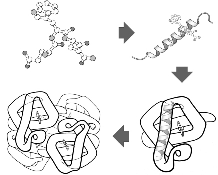
TABLE 2.2 Functional Relevance of Quaternary Structure

Interestingly, most proteins are folded such that aggregation with other polypeptides is avoided (Richardson, 1992); the formation of multisubunit proteins is therefore a very specific interaction. Quaternary structures are stabilized by the same types of interactions employed in tertiary and secondary structure stabilization. The surface regions involved in subunit interactions generally resemble the cores of globular proteins; they consist of residues with nonpolar side chains, residues that can form hydrogen bonds, or residues that can participate in disulfide bonds. Table 2.2 explains some of the functional advantages that are bestowed upon proteins by their quaternary structure.
Protein structure is complex, but it should be noted that by the 1970s protein scientists had determined most of the basic principles. These findings were confirmed in later years, as the pace of protein structure determination increased. These basic principles of protein structure now form the stable foundation needed for researching many of the remaining questions in protein science.
Computational tools now available, and described throughout this book, make management of the complexity of protein structure information more tractable. Protein structures can be more easily determined (see Chapter 40), and hypotheses as to the nature of protein structure can be more easily tested. As a result, it is now possible to pose more sophisticated questions, and in the coming years protein scientists can look forward to an understanding of protein structure and function on a much deeper level.
MORE INFORMATION ON THE INTERNET
The RCSB Protein Data Bank (PDB): http://www.rcsb.org/. [The sole worldwide public repository for macromolecular structure data.]
Education Resources Listing at the PDB. [A collection of links to educational resources covering protein structure.]
TOPS homepage and server: http://www.tops.leeds.ac.uk. [Used to create one of the figures in this chapter.]
MolScript homepage: http://www.avatar.se/molscript/. [A popular package for generating images of protein structure, used to create many of the figures in this chapter.]
PyMol homepage: http://pymol.sourceforge.net. [A popular package for generating images of protein structure, used to create figures in this chapter.]