20
IDENTIFYING STRUCTURAL DOMAINS IN PROTEINS
INTRODUCTION
Analysis of protein structures typically begins with decomposition of the structure into more basic units called structural domains. The underlying goal is to reduce a complex protein structure to a set of simpler, yet structurally meaningful units, each of which can be analyzed independently. Structural semi-independence of domains is their hallmark: domains often have compact structure that can fold (and sometimes function) independently. The total number of distinct structural domains is currently hovering around one thousand: they are represented by the unique folds in SCOP classification (Murzin et al., 1995) or unique topologies in CATH classification (Orengo et al., 1997). Interestingly, this is what Chothia predicted at a rather early stage of the Structural Genomics era (Chothia, 1992).
A significant fraction of these domains is universal to all life forms, others are kingdom-specific and yet others are confined to subgroups of species (Ponting and Russell, 2002;Yang, and Doolittle, and Bourne, 2005). The enormous variety of protein structures is then achieved through combination of various domains within a single structure. This “combining” of domains can be achieved by combining together single domain polypeptide chains within a noncovalently linked structure or by combining domains (via gene fusions/ recombination) on a single polypeptide chain that folds into the final structure (Bennett, Choe, and Eisenberg, 1994). There are benefits to both strategies: the former can be seen as a more economic and modular approach in which many different structures can be put together with relatively few components within the cell. The latter, combining a specific set of modules within a single polypeptide chain, ensures that they are expressed together and localized in the same cells or cellular compartments (Tsoka and Ouzounis, 2000). This chapter is concerned with this latter case: the decomposition of the multidomain polypeptide chain into structural domains.
Sequence information is often insufficient for identifying structural domains in the protein because the same structure can be reached from widely divergent sequence space (typically down to 30% sequence identity). Therefore, knowledge of protein structure is often a prerequisite to the delineation of structural domains. With the current rapid increase in the number of solved structures, a fast and consistent delineation of structural domains has great potential as well as great importance. Yet, in spite of the attention given over the last 30 years to the problem of domain delineation, it is not completely resolved as of today. While there are many methods for domain identification, the consistency of agreement among methods is 80% or less with the complex multidomain structures presenting most of the challenges (Holland et al., 2006). Some of the methods for domain identification are based exclusively, or partially, on the knowledge of human experts, while the other ones (computational methods) attempt to solve this problem in a completely automated way (Veretnik et al., 2004; Veretnik and Shindyalov, 2006). Expert methods are nearly always superior to the computational methods because experts can employ myriads of algorithms based on prior knowledge, biological and structural sensibility that ultimately will lead to a structure partitioning which might be inconsistent with some of the prior cases. Computational methods, on the contrary, are not able to reconcile the contradictions within the structural data set that might be internally inconsistent due to its biological complexity. Hence, current computational methods have difficulties in defining domain boundaries if the new examples require ingenious solutions that are contradictory to those previously acquired. The advantage of computational methods, however, is that they are fast and consistent—a feature of great importance in the era of structural genomics.
This chapter presents an overview of computational methods for parsing experimentally determined protein 3D structures into structural domains. The basic concepts underlying the domain parsing methods have been developed nearly 30 years ago, and has changed little since then. The actual algorithms, on the contrary, have undergone some new developments recently in terms of speed, generality, as well as fine-tuning. More important still, because of the increased complexity of the structures solved, we know much more today about the world of protein folds and their diversity. This makes the domain assignment problem more challenging, yet it also provides a broader data set of structures for tuning/improving algorithms. Before proceeding, we make a short note on terminology: the terms “partitioning,” “delineation,” “decomposition,” “cutting,” and “assignment” are used interchangeably here and have no special meaning associated with a particular term when referring to the partitioning of a protein chain into structural domains.
DEFINITIONS OF STRUCTURAL DOMAINS
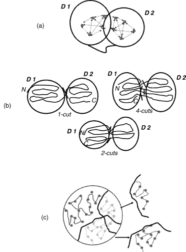
Structural domains can be thought of as the most fundamental units of the protein structure that capture the basic features of the entire protein. Among such features are (1) stability, (2) compactness, (3) presence of the hydrophobic core, and (4) ability to fold independently. These structural/thermodynamic properties of domains suggest that atomic interactions within domains are more extensive than that between the domains (Wetlaufer, 1973; Richardson, 1981). From this, it follows that domains can be identified by looking for groups of residues with a maximum number of atomic contacts within a group, but a minimum number of contacts between the groups, as illustrated in Figure 20.1a. The spatial compactness of domains sometimes results in noncontiguous domains where stretches of residues that are distant on the polypeptide chain are found in close proximity in the folded structure (Figure 20.1b). This situation may arise as a result of gene insertion events or domain swapping (Bennett, Choe, and Eisenberg, 1994). Domains are the building blocks of the proteins: different combinations of domains result in variety of protein structures. Frequently, domains are associated with specific functions, such as binding a ligand, DNA or RNA or interacting with other protein domains.
Figure 20.1. Illustration of the problem of parsing the protein 3D structure into structural domains. (a) Most commonly, structural domains are defined as groups of residues with a maximum number of contacts with in each group and a minimum number of contacts between the groups. Domains may be composed of one or more chain segments. Any domain assignment procedure must therefore be able to cut the polypeptide chains asmanytimes as necessary. (b)When both domains are composed of contiguous chain segments (continuous domains), only a one-chain cut (1-cut) is required. When one domain is continuous and the other discontinuous, a situation that may arise as a result of gene insertion, then the chain has to be cut in two places (2-cuts).When both domains are discontinuous, additional chain cuts may be required. In the example shown, the chain is cut in four places (4-cuts), and thus the domain on the left hand side contains three chain segments, whereas that on the right contains two chain segments.(c) This drawing shows two solutions to the problem of partitioning the protein 3D structure into substructures. To partition the 3D structure into domains, many such solutions need to be examined to single out the one that satisfies the criterion given in (a). Figure also appears in the Color Figure section.
ALGORITHMS FOR IDENTIFYING STRUCTURAL DOMAINS: INSIGHT INTO HISTORY AND METHODOLOGY
Using the above definitions for domains as guidelines, systematic partitioning of structures into domains has been undertaken. This task can be done manually by experts in protein structure or automatically by encoding basic rules and assumptions in an algorithm. The former has the advantage of employing human expertise with myriads of algorithms integrating prior experience, common sense, topological sensibility, and other knowledge. The latter, while far less sophisticated, has the advantage of speed and consistency that are critical in the current era of structural genomics, when the sheer number of solved structures overwhelms human experts.
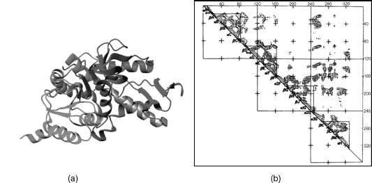
The first manual survey of structural domains in proteins was carried out nearly 30 years ago (Wetlaufer, 1973) using visual inspection of the then-available X-ray structures. Wetlaufer defined domains as regions of the polypeptide chain that form compact globular units, sometimes loosely connected to one another. At about the same time, the first so-called Cα-Cα distance plots were computed (Phillips, 1970; Ooi and Nishikawa, 1973) and shown to be useful for identifying structural domains. Domains were identified visually in these plots by looking for series of short Cα-Cα distances in triangular regions near the diagonal, separated by regions outside the diagonal where few short distances occur, as illustrated in Figure 20.2. Manual and semimanual surveys became more extensive and systematic after 1995; currently there are three major sources of information regarding domains: SCOP (Murzin et al., 1995, Chapter 17), AUTHORS (Islam, Luo, and Sternberg, 1995), and CATH (Orengo et al., 1997, Chapter 18). We will discuss the evaluating procedure for domain assignment later in the chapter.
Figure 20.2. Domain structure of dogfish lactate dehydrogenase, determined using the Cα–Cα distance map. (a) Ribbon diagram of lactate dehydrogenase, showing the NADbinding (green) and catalytic domains (red). In gray is part of the helix, spanning residues 164–180, linking the two domains. (b) Distance map and structural domains in lactate dehydrogenase. Contours represent Cα–Cα distances of 4, 8, and 16Å within the subunit of dogfish lactate dehydrogenase. Elements of secondary structure are identified along the diagonal. Triangles enclose regions where short Cα–Cα distances are abundant. The NAD binding domain comprises the first two triangles (counting from the N-terminus) that are subdomains. The catalytic domain comprises the last two triangles (the Cterminal domain). Taken from Rossman and Liljas (1974) and reproduced by permission of Academic Press (London) Ltd. Figure also appears in the Color Figure section.
Rossman and Liljas performed the first systematic algorithmic survey of domains for a set of protein 3D-structures (Rossman and Liljas, 1974) by analyzing Cα-Cα distance maps. This was followed a few years later by three other studies conducted by Crip-pen (1978) and Rose (1979) and by Wodak and Janin (1981b), and Janin and Wodak (1983) (Table 20.1). The methods described in these studies involved different algorithms and produced different results, but had one major aspect in common: the protein 3D structure was partitioned in a hierarchical fashion that yields domains and smaller substructures, as illustrated in Figure 20.3. Surveys of these smaller substructures in a set of proteins revealed recurrent structural motifs comprising of two or three secondary structure elements joined by loops (Wodak and Janin, 1981a; Zehfus and Rose, 1986). Interestingly, the systematic identification of similarly defined smaller sub structures in proteins was recognized year later as a useful way for predicting region in protein that would form first during folding (nucleation sites) (Moult and Unger, 1991; Berezovsky, 2003). Over 20 different algorithmic approaches have been applied to this problem in the sub sequent three decade (this survey cover method up to 2007). The overarching theme of structural partitioning is based on contact density, that is , the simple fact that there are more residue-to-residue contact within a structural unit than between the structural unit . The implementation of this principle can be very different in different method a can be seen in Table 20.1, but the underlying idea always comes back to finding regions with a high density of interaction.
Figure 20.3. Illustration of the hierarchic partitioning of protein 3D structures into substructures performed by three of the early automatic domain analysis methods. (a) The partitioning procedure of Rose et al. (1979) is applied to dogfish lactate dehydrogenase. The chain tracing of the subunit is projected into a “disclosing plane” passing through its principal axes of inertia. A line is then found that divides the projection into two parts of about equal size. The different projections represent (from left to right and from the bottom down) the whole subunit (residues 1–331) of the N-terminal domain (1–161) and the subdomain (residues 1–90 and 1–49). Taken from Rose (1979) and reproduced with permissionof Academic Press (London) Ltd. (b) Domain andsubdomain hierarchies in concanavalin A adapted from Crippen (1978). It represents an ascending hierarchy of clusters starting from 13 “reasonably straight segments” at the bottom of the hierarchy and culminating with the entire concanavalinAsubunit. (c) The domain and subdomain hierarchy in concanavalin A, adapted from Wodak and Janin (1981b). It describes the descending hierarchy derived from identifying the minimum interface area between substructures in successive interface area scans. Unlike the hierarchy in (b), this one generates continuous substructures. The agreement with the hierarchy in (b) is therefore poor.
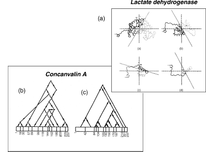
TABLE 20.1. Summary of Domain Decomposition Methods 1974–2007
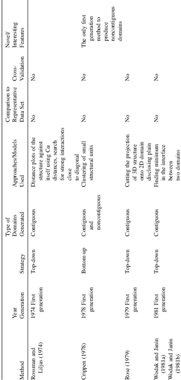
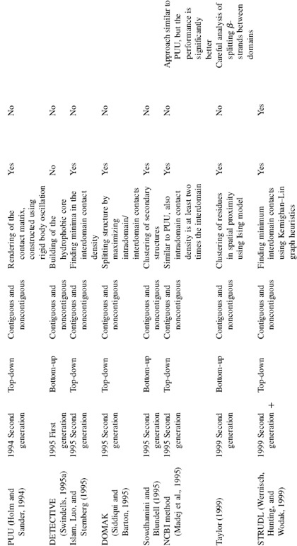
Methodologically, algorithms can be separated into first generation: methods published during the period 1974—1995; and second generation algorithms: methods published from 1994 until now. The first generation of algorithms was based on a very limited set of available structural data at the time thus, some rather general principles were difficult to capture due to the paucity of structural examples. For the same reason, neither a systematic comparison against a representative data set nor separation of the data into training and testing subsets was possible until the middle 1990s. The second generation methods, which began around 1994, relied on a large set of structures for training and they routinely compare performance of the algorithm against a representative data set, typically assigned by human experts. Surprisingly, the methodological rigor is often absent and the algorithms are often trained and tested on the same set of data. Methods that incorporated cross-validation to test the algorithm during development by using nonoverlapping training and testing data sets are more balanced in their approach and we assign them as “second generation +” (Table 20.1). The majority of the second generation methods are able to deal with noncontiguous domains (Zehfus, 1994).
Domain identification can be divided into two fundamental approaches: top-down (starting from the entire structure and proceeding through iterative partitioning into smaller units) and bottom-up (defining very small structural units and assembling them into domains). Some methods use both the approaches within their algorithm by first decomposing the structure and then reassembling them, or vice versa. Here, we classify each method based on its chief or overall approach to the domain identification. Generally, the process of domain decomposition is performed in two steps: (1) tentative domains are constructed either by splitting the structure into domains or building domains from smaller units; (2) these tentatively defined domains are evaluated in a postprocessing step. Overall, an amazing array of approaches has been put forward over the years to solve the domain decomposition problem; the strategies vary from maximizing intradomain contacts to minimizing domain—domain interface, from semi-independent motion of domains to clustering residues in spatial proximity. Other techniques applied for domain definition come from graph theoretical approaches (i.e., Kernighan—Lin graph heuristics, Network flow, Delaunay tessellation), rigid body oscillation, spectral analysis, Ising model, Gaussian Network Model, and so on (Table 20.1). In spite of this variety of approaches and techniques, an interesting observation emerges when one carefully compares the performance of the algorithms: most of the algorithms solve correctly 70—80% of the available structures, faltering on the remaining ones because of their complex, multidomain structures. Typically, all methods correctly identify potential boundaries between the structurally compact regions. However, in some cases the number of boundaries are overpredicted leading to too many assigned domains (overcut) or underpredicted leading to fewer assigned domains (undercut). Thus, the problem still remaining is not “where does the boundary of domains fall?”, but rather “is the identified boundary a true domain boundary?” Some of the difficulties come from very complex and contradictory scenarios that are presented by existing protein structures, making it nearly impossible to capture by a simple set of rules. This, in turn, is part of the complexity inherent in biology in general. In this case, complexity arises in that some domains are not globular, lack a hydrophobic core in the absence of the binding partner, have relatively low intradomain contact density, or have extensive interactions along the domain—domain interface. Identifying a correct subset of domain boundaries from the set of potential boundaries is the next (and maybe the final) frontier in solving the domain assignment problem for structures.
ALGORITHMS FOR IDENTIFYING STRUCTURAL DOMAINS: IN-DEPTH
Of the more recent second generation methods for domain assignment, several make elegant use of graph theoretical methods. In this section, we discuss two such methods that use somewhat different techniques to address the problem of partitioning protein structure into structurally meaningful domains. First, we will discuss STRUctural Domain Limits (STRUDL) (Wernisch, Hunting, and Wodak, 1999) followed by DomainParser (Guo et al., 2003).
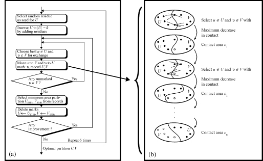
The procedure implemented in STRUDL views the protein as a 3D graph of interacting residues, with no reference to any covalent structure. The problem of identifying domains then becomes that of partitioning this graph into sets of residues such that the interactions between the sets is minimum. Since, this problem is NP-hard, efficient heuristic procedures—procedures capable of approximating the exact solution with reasonable speed—are an attractive alternative. The algorithm used in this case was a slightly modified version of the Kernigan—Lin heuristic for graphs (Kernighan, 1970). The application of this heuristic to domain assignment is summarized in Figure 20.5.
A useful, though not essential, aspect of this application is that the interactions between residue subsets were evaluated using contact areas between the atoms. This area was defined as the area of intersection of the van der Waals sphere around each atom and the faces of its weighted Voronoi polyhedron. This contact measure is believed by the authors to be more robust than counting atomic contacts due to its lower sensitivity to distance thresholds.
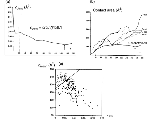
To identify domains for which the limits and size are not known in advance, the partitioning procedure described in Figure 20.4 is repeated k times, with k representing all the relevant values of the domain size, ranging from 1 to N/2, and N being the total number of residues in the protein. The partition with minimum contact area, identified for each value of k, is recorded. This information is then used to compute a minimum contact density profile. In this profile, the minimum contact area found for each k is normalized by the product of the sizes of the corresponding domains, to reduce noise (Holm and Sander, 1994;Islam, Luo, and Sternberg, 1995) and plotted against k. The domain definition algorithm then searches for the global minimum in this profile. Figure 20.5a illustrates the profile obtained for a variant of the p-hydroxy-benzoate hydroxylase mutant (PDB-RCSB code 1dob), a 394-residue protein composed of two discontinuous domains. The global minimum in the minimum contact density profile, although quite shallow, is clearly visible at k = 172, and yields the correct solution. The corresponding partition cuts the chain in five distinct locations yielding two domains, comprising six chain segments. The smaller of the two domains contains 172 residues; the largest contains 222 (394—172) residues.
Figure 20.4. Domain identification using the graph heuristic procedure implemented in STRUDL (Wernisch, Hunting, and Wodak, 1999). (a) Overview of the major steps in the STRUDL algorithm (b) The residue exchange procedure in STRUDL. Residues u ε U and v ε V (filled circles) are selected so as to produce a maximal decrease or, if that is not possible, a minimal increase in the contact area between U and V upon exchange. Once moved to V, residue u is flagged (empty circle) and can hence not be moved back to U. The exchange procedure stops when V contains only flagged residues. Among all partitions with contact area Ci, with i=0, . . ., n the one with minimum contact area Cmin is selected.
Once the global minimum is identified in the minimum contact density profile,a decision must be taken to either accept or reject the corresponding partition, with a rejection corresponding to classifying the structure as a one-domain protein. An obvious criterion on which to base such decision is the actual value of the contact area density in profiles such as that of Figure 20.5 a. If this value is below a given threshold, the partition is accepted; otherwise, it is rejected. But this simple criterion is unfortunately not reliable enough. Following other authors, additional criteria that represent expected properties of domains and of the interfaces between them were therefore used to guide the decision (Rashin, 1981; Wodak and Janin, 1981b). The choice of these criteria was carefully optimized on a training set of 192 proteins using a discriminant analysis, and tested on a different, much larger set of proteins, as summarized in Figure 20.5c. Finally, once a partition is accepted, the entire procedure is repeated recursively on each of the generated substructures until no further splits are authorized. This recursive approach was shown to successfully handle proteins composed of any number of continuous or discontinuous domains.
As always, assessing the performance of the method is a crucial requirement. Fortunately, the significant increase in the number of different proteins of known structure presently offers a more extensive testing ground. STRUDL was applied to a set of 787 representative protein chains from the PDB (Bernstein et al., 1977; Berman et al., 2000), and the results were compared with the domain definitions that were used as the basis for the CATH protein structure classification (Orengo et al., 1997). This definition was based on a consensus definition produced by Jones et al. (1998) using three automatic procedures, PUU (Holm and Sander, 1994), DETECTIVE (Swindells, 1995a), and DOMAK (Siddiqui and Barton, 1995), as well as by manual assignments. Results showed that domain limits computed by STRUDL coincide closely with the CATH domain definitions in 81% of the tested proteins and, hence, that it performs as well as the best of the above-mentioned three methods. In contrast to these methods, however, it uses no information on secondary structures to prevent the splitting P-sheets, for instance. The 19% or so protein for which the domain limits did not coincide, represent interesting cases which could, for the most part, be rationalized either on the basis of the intrinsic differences between the approaches (in this case, STRUDL versus CATH) or by the variability and complexity inherent in real proteins.
Figure 20.5. Parameters used to partition and/or to evaluate domain partitioning in STRUDL. (a) The minimum contact density profile for the p-hydroxy-benzoate hydroxylase mutant (1DOB). The Cdens value in Å, is computed using the formula given in the figure. In thisformula, c(U,V) is the contact area between the two residue groups U and V, and IUI and IVI are the number of residues in U and V, respectively. The plotted values represent the minimum of Cdens computed for a given domain size k, where k = 1, N/2, with N being the total number of residues in the protein chain. Hence IUI and IVI equal k and N-k, respectively. The arrow at k = 172 indicates the global minimum of this profile. The dashed line delimits the value of k = 20 below which splits are not allowed to avoid generating domains containing less than 20 residues. (b) The profiles of minimum contact area c(U, V) in Å computed as a function of k, the number of residues in the smallest substructure U, for the same protein as in (a). Shown are the profile with no constraints on the number of chain cuts, as in the STRUDL procedure, and four other p-cut profiles, obtained by limiting the number of allowed chain cuts p (see Wernisch et al., 1999 for details). Those are 1-cut (- - -), 2-cuts (- - -), 3-cuts (- - -), and 4-cuts(...). The global minimum of the contact area (arrow) can only be located in the unconstrained profile, illustrating the advantages of STRUDL over other procedures in which the number of allowed chain cuts is fixed. (c) Plot ofthe mean burial bmean in A, versus the contact area ratio cprop. Both quantities are evaluated for domain partitions corresponding to the global minimum in the contact area density profiles computed by STRUDL. bmean is the average interresidue contact area of a given substructure. Cprop isthe ratio of the contact area of the putative domains to the sum of the inter residue contact areas in the entire proteins. The straight line optimally separating the single (filled circles) from the multidomain proteins (empty circles). This optimal separation entails however, 19 errors—proteins classified in the wrong category—out of the total of 192 protein considered in the set.
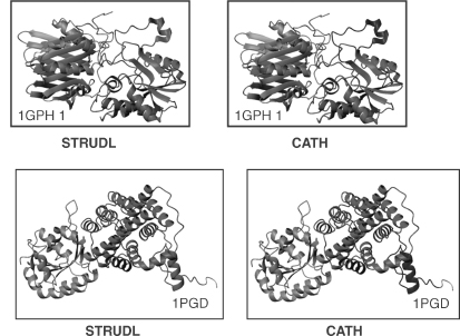
Several of these cases are illustrated in Figures 20.6 and 20.7. Figure 20.6 shows cases where STRUDL splits proteins into two domains that are considered a single architecture by CATH. Among the shown examples are the DNA polymerase processivity factor PCNA (1PLQ), which clearly shows an internal duplication, and the lant seed protein narbonin (1NAR), which adopts a TIM barrel fold that many automatic domain assignment procedures tend to split into two domains. Differences of this type could be rationalized by the fact that CATH imposes criteria based on chain architecture and topology, whereas STRUDL does not. Figure 20.7 illustrates two cases, where the results of STRUDL and CATH differ by the assignment of a single relatively short protruding chain segment. Such cases illustrate the inherent noisiness in the backbone chain trace, which invariably affects domain assignments.
Domain Parser uses a top-down graph theoretical approach for domain decomposition and an extensive postprocessing step. During the training stage of the algorithm, multiple parameters are tuned; the method is then validated on a SCOP data set. Domain decomposition is addressed by modeling the protein structure as a network consisting of nodes (residues) and edges (connections between residues). A connection between any two residues is drawn when they are adjacent in the sequence or, alternatively, are in physical proximity in the structure. The strength of the interaction between two residues is expressed as the capacity of the edge to connect the two nodes. This edge capacity is a function of (a) the number of atom—atom contacts between residues; (b) the number of backbone contacts between residues; (c) the existence of backbone interactions across a beta-sheet; and (d) whether both residues belong to the same beta-strand. The values for all parameters involved in edge capacity are optimized during the training stage of the algorithm.
Figure 20.6. Examples of single domain, single architecture proteins in CATH (Jones et al., 1998), which STRUDL (Wernisch, Hunting, and Wodak, 1999) splits into two domains. Shown are the domain assignments produced by STRUDL. For the exact domain limits, the reader is referred to the STRUDL Web site. The displayed protein ribbons belong to Torpedo californica acetylcholinesterase monomer (1ACE), the lant seed protein narbonin (1NAR), the eukaryotic DNA polymerase processivity factor PCNA (1PLQ), and Chorismate mutase chain A monomer (1CSM_A).
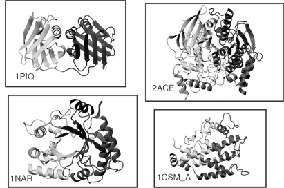
Figure 20.7. Different assignments by STRUDL (Wernisch, Hunting, and Wodak, 1999) and CATH (Jones et al., 1998), illustrating the effect of “noise,” or decorations, in the protein chain trace. The STRUDLassignments are displayedonthe left hand side, and the CATH assignments are displayed on the right. The short chain segments, which CATH assigns to separate domains, are shown in blue. Some of the discrepancies may be due to simple “slips” in the CATH assignments that have been, or will be, corrected. Figure also appears in the Color Figure section.
The partitioning of the network into two parts is then equivalent to decomposing a given structure into two domains. Ideally, partitioning should be done using the edges with least capacity, which will result in partitioning a structure along the least dense interactions among the residues. The problem of partitioning the network is solved using the maximum flow/ minimum cut theorem by Ford—Fulkerson as implemented by Edmond and Karp. Briefly, the approach is as follows: artificial source and sink nodes are added to the network (Figure 20.8a). A “bottleneck”—a set of critical edges in the network flow—is found by gradually increasing the flow of all edges in a network. Removing the set of critical edges from the network prevents flow from the source to the sink. At this point, nodes that are connected to the source represent one interconnected part of the network, while nodes connected to the sink are the second interconnected part of the network. Since the node capacity is increased gradually, it is expected that nodes with least capacity (least residue— residue contacts) will be the ones contributing to the bottleneck. The process of subdividing the network into two parts is repeated multiple times by connecting the source and sink to different parts of the network; a set of minimal cuts is collected and evaluated during a postprocessing step. The entire procedure is then repeated in each of the resulting domains until either the domain’s size drops below 80 residues or the partitioning produces domains that do not meet necessary conditions of domain definitions.
Figure 20.8. Domain decomposition using the DomainParser algorithm. (a) Schematic representation of protein structure as a directedflownetwork. The value on each edge represents the edge’s capacity. Artificial nodes “start” and “sink” are denoted by s and t, respectively. (b–g) are examples of parameters used by the algorithms. (b) zero- and second-order spherical moment profile of structure 2ilb, (c) compactness of structure, (d) size of the domain interface relative to the domain’s volume, (e) measure of relative motions between domains, (f) distribution of the number of segments per domain, and (g) distribution of domain sizes. (h) Neural network architecture for evaluation of decomposed individual domains.
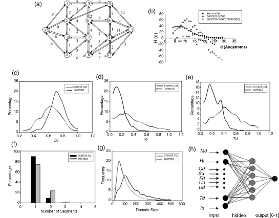
The stopping criteria are multifaceted and defined by (1) domain size (no less than 35 residues), (2) beta-sheets kept intact, (3) compactness of domain above threshold gm, (4) size of the domain—domain interface below threshold fm, (5) the ratio of the number of residues and the number of segments in the domain is above threshold ls. The values for gm,fm, ls and minimum domain size are determined during the training stage of the algorithm. A suite of additional parameters exists—these are involved in a postprocessing step of the algorithm in which an assessment is made about whether the substructure meets the additional criteria of a structural domain. These parameters are (1) hydrophobic moment (Figure 20.8b), (2) the number of segments in the partitioned domain (Figure 20.8f), (3) compactness (Figure 20.8c), (4) the size of domain interface relative to the domain’s volume (Figure 20.8d), and (5) relative motion between compact domains (Figure 20.8e). Distribution for each of the parameters for true versus false domains is collected during the training stage using 633 correctly partitioned domains and 928 incorrectly partitioned domains. Multiple neural networks are then investigated; the best one has nine input nodes, six nodes in the hidden layer, and one output node (Figure 20.8h). Performance of the DomainParser method is then evaluated using a set of 1317 protein chains in which domains are defined by SCOP.
DOMAIN ASSIGNMENTS: EVALUATING AUTOMATIC METHODS
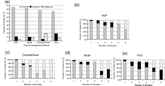
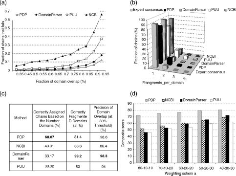
A chief reason for the existence of over two dozen methods for domain decomposition is the complexity of the problem itself: it is nearly impossible to capture succinctly the principles of domain decomposition and apply them successfully to the entire universe of protein structures. Thus, every new method strives to reach a bit further beyond existing methods in its ability to decompose complex structures. With so many different methods available, it is essential to be able to compare the performance of the algorithms, to determine the fraction, as well as the type, of successfully partitioned proteins. Evaluation of automatic methods is an essential part of algorithm development process and the performance of a method is often reported in the second generation of algorithms. To evaluate the performance of a new domain assignment method, authors usually apply it to a set of proteins for which experts who are either crystallographers or protein classifiers have produced domain assignments manually. However, authors of each method use different data sets for evaluation of their algorithms; thus, it is nearly impossible to cross-compare the performance of various methods. Only one consistent benchmark data set existed until recently and it is a set of 55 protein chains consistently assigned by Jones et al. (1998). This data set was assembled by finding a consensus using the Islam et al. data set among four automatic methods: PUU (Holm and Sander, 1994), DETECTIVE (Swindells, 1995b), DOMAK (Siddiqui and Barton, 1995), and the method developed by Islam, Luo, and Sternberg (1995). For the evaluation, any two assignments (one from the benchmark set, another by the algorithmic method) were considered similar if they had the same number of domains and at least 85% of the residues were assigned to the same domain. Fifty-five proteins is a very small benchmark set, thus it is likely that its resolution will be insufficient to detect differences between the methods. New benchmark data sets were compiled recently (Veretnik et al., 2004; Holland et al., 2006) specifically for the purpose of cross-comparing the performance of the algorithms as well as highlighting the strengths and weaknesses of each algorithmic method. The data set is assembled using a principle of consensus approach among the human experts: it includes proteins for which three expert methods (CATH, SCOP, and AUTHORS) produce similar domain decompositions. Such consensus approach eliminates the more complicated structures for which no agreement can be reached among human experts. This fraction of “controversial” proteins is intentionally left out, so as not to further complicate the issue. The 315 proteins in this new benchmark (Benchmark_2 in Holland et al., 2006) are realistically distributed between single-domain and multidomain proteins to avoid the typical bias toward one-domain proteins (Table 20.2). Furthermore, each type of topology combination, as determined by CATH classification on the level of Topology, occurs only once per data set to ensure that a broad range of topologies found in the protein universe are equally represented. The above benchmark data set was used to evaluate four recent publicly available automatic methods: PUU (Holm and Sander, 1996), DomainParser (Xu, Xu, and Gabow, 2000; Guo et al., 2003), PDP (Alexandrov and Shindyalov, 2003), and NCBI (Madej, Gibrat, and Bryand, 1995). The evaluation includes information about the success rate of each al gorithm and an analysis of errors in terms of predicting fewer domains (undercut) or too many domains (overcut) (Figure 20.9a). A more scrutinized examination was also conducted by inspecting (1) the performance of domain boundary prediction for each example of multidomain structures (Figure 20.9b—e), (2) tendencies for methods to fragment domains into noncontiguous stretches of polypeptide chain (Figure 20.10a), and (3) the precision of overlap of domain boundaries (Figure 20.10b).
TABLE 20.2. Benchmark Data Sets Constructed for Evaluation of Computational Methods for Domain Assignments from 3D Structure
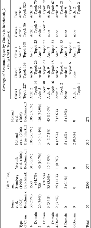
Figure 20.9. Comparison of the performance of domain assignment methods using Benchmark_2 data set (built on the principle of consensus among expert-based assignments:expert consensus).Four currently available algorithmicmethods are evaluated:DomainParser, PDP, PUU, and NCBI. Structure is considered to be assigned correctly if the algorithm predicts the same number of domains as predicted by expert consensus. Correctly assigned structures are represented in grey, structures with too many assigned domains (overcut) are in black, and the structures with too few domains (undercut) are indicated by the dotted pattern. (a) Performance of each method on the entire Benchmark_2 data set. (b–e) Performance of individual methods on structures grouped by the number of domains they contain. (b) PDP method. (c) DomainParser method. (d) NCBI method. (e) PUU method.
Finally, a composite evaluation that accounts for the correct number of domains, fragments, and domain boundary assignment can be a more comprehensive approach to conducting a cross-comparison of performances of various algorithms (Figure 20.10c and d). By changing the weighing schema of individual performance components of the methods, it allows for comparisons to be conducted from different angles that stress particular features of interest. In our analysis, the PDP method is a clear winner regardess of the weight that is attributed to individual parameters. On the contrary, the performance of DomainParser improves to the point of out performing the NCBI method when a higher weight is given to the precision of boundaries rather than prediction of the correct number of domains.
This type of systematic ana ysis can ink performance of an a gorithm in terms of its strength and weaknesses to particu ar assumptions found in the a gorithm, as we as to the specific data sets on which algorithms had been trained. For example, the superior performance of PDP can be partially linked to its ability to cut through secondary structures, particularly β-sheets, and assign them to different domains. This particular property is interpreted differently in all other tested methods. On the contrary, a complete “taboo” on cutting any secondary structure element, as imposed in the NCBI method, results in poorly matched domain boundaries in cases where the proper domain boundaries do occasionaly fall within secondary structure elements rather than loops. A tendency toward very compact domains forces the PUU algorithm to build domains out of many discontinuous fragments that often do not make sense from the evolutionary perspective. Rigorous tuning of multiple parameters in the DomainParser algorithm results in excellent prediction on the level of domain boundaries and the number of domain fragments, but at the same time it produces a large fraction of undercut structures. This might partially be due to the training and testing data set that is based on SCOP, an expert database with significant level of undercut predictions compared to CATH and AUTHORS. Another issue is that the threshold for splitting β-strands and β-sheets might be set incorrectly. In summary, analysis ofalgorithm performance offers both a relative ranking of the methods among themselves as well as insights into particular areas of difficulties for each method; these may lead to new insights and further improvements.
Figure 20.10. Comparison of the performance of domain assignment methods using Benchmark_2.(a) Evaluation of correct placement of domain boundaries using different levels of stringency of overlap of the predicted domain assignment and expert consensus assignment. Asstringency of overlap increases, a larger fraction of structures fails the domain overlap test. (b) Evaluation of assignment of noncontiguous domains by different methods. Most of the methods predict more noncontiguous domains than experts. (c) Performance of each method using three main criteria: (1) fraction of structures with correctly assigned number of domains, (2) correctly assigned noncontiguous domains, and (3) correct placement of domain boundaries (at 80% precision threshold). (d) Composite evaluation of performance, which combines three components described in (e) , using different weighting schema. The firstcomponent inthe schemais the fraction of correctly assigned domains; second component: correctly fragmented domains; third component: correct placement of domain boundaries (at 80% precision threshold). Regardless of the weighting schema, PDP always appears the best method, while PUU is worse. The performance of DomainParser improves significantly when a larger weight is given to correct fragmentation and boundary placement, so that eventually it surpasses the performance of NCBI method.
DOMAIN PREDICTION BASED ON SEQUENCE INFORMATION
Identifying protein domains by using only sequence information is even a more challenging task. However, this approach is not limited to proteins with solved 3D structures. For the vast majority of protein sequences, the structure is unknown thus, sequence-based methods are of great importance and, indeed, this area of research is very active. The detriments of predicting boundaries of structural domains without knowing the structure are (1) the level of correct assignments is lower than that for structure-based methods; this difference becomes particularly sharp in the cases of multidomain proteins with complex architectures, and (2) only a few of the sequence-based methods can predict noncontiguous domains that constitute about 10% of all domains (Holland et al., 2006). There is almost no overlap or collaboration between sequence-based and structure-based methods, as we will see from terminology and evaluation methods. The very subject of prediction of structural domains is coached here in terms of predicting domain boundaries.
Sequence-based methods can be divided into several categories: (1) prediction in the absence of sequence information, (2) methods that use information from single sequence (when no homologous sequences are available), (3) methods based on multiple homologous sequences, and (4) methods that incorporate structure prediction from sequences.
Algorithms Based Purely on Domain and Protein Sizes
“Domain Guess by Size” (DGS) (Wheelan, Marchler-Bauer, and Bryant, 2000) is an example of an algorithm that does not use any sequence or structure information. Rather, it predicts protein partitioning based exclusively on the size of the protein. The algorithm predicts several probable outcomes by using likelihood functions based on empirical distributions of protein length, domain length, and segment number as observed in the PDB. This is the only method in the sequence-based category that can predict noncontiguous domains. DGS identifies domain boundaries with 57% accuracy and an error margin of ±20 residues for two-domain proteins. If proteins were simply chopped in half, this approach will only yield an 8% success rate.
Algorithms Based on Single Sequence Information
When prediction of domain boundaries is based on a single sequence, the amino acid propensity is typically calculated for linker regions associated with domain boundaries. Each residue in the sequence is scored with linker index to construct a linker profile and boundaries are identified with a threshold for the scores. DOMcut (Suyama and Ohara, 2003) identifies domain linkers with 53.5% sensitivity and 50.1% selectivity using a linker index deduced from a data set of domain/linker segments. Armadillo (Dumontier et al., 2005) uses a linker index enhanced by positional confidence scores leading to a performance of 56% and 37% sensitivity for two- and multidomain proteins, respectively. These simple strategies indicate that amino acid propensities in linker regions are distinct and differ from the rest of the protein. Such potential patterns in linker regions have further been exploited by using more advanced machine learning techniques such as neural networks. CHOPnet (Liu and Rost, 2004b), PPRODO (Sim 2005), and a newly developed neural network (Ye et al., 2008) report ~69% accuracy for two-domain proteins.
Algorithms Based on Multiple (Homologous) Sequences
The challenges of identifying boundary regions are diminished when there is detectable sequence homology to the characterized domains. Several algorithms use linkages between the similarities in sequences such as CHOP (Liu and Rost, 2004a). These similar sequences can also be aligned to generate multiple sequence alignments (MSA) that are subsequently analyzed to identify domain boundaries. Domaination (George and Heringa, 2002a) is an example of an algorithm that analyzes features in the MSA to partition proteins into domain units. Nagarajan et al. developed an approach to identify transition positions between domains within the MSA using several probabilistic models (Nagarajan and Yona, 2004). Clustering of the sequences is also a popular approach in identifying domains and is a strategy employed by DIVCLUS (Park and Teichmann, 1998), MKDOM (Gouzy, Corpet, and Kahn, 1999), and ADDA (Heger and Holm, 2003). Finally, the use of taxonomic information has been shown to be useful to help identify domains as well (Coin, Bateman, and Durbin, 2004).
Adding Predicted Structure to Sequence Prediction
While domain identification can be achieved using a purely sequence-based strategy, the use of structural information either integrated during the training or prediction process when developing sequence-based domain identification can impart added advantage. As an example, a comparison between the sequence and structural alignments of domains illustrates the added advantage of using the information content inherent in structural data leading to an improvement over sequence alignments (Marchler-Bauer et al., 2002). We will discuss the strategies that have been employed to improve sequence-based identification of domains and highlight how the use of structural data has been helpful in the development of these tools.
Incorporating ab initio structure prediction, either at the secondary or tertiary structure level, has also been used to identify domain boundaries. Sequence-based secondary structure predictors have reached performances as high as 78% accuracy and can be used to help delineate domain boundaries. DomSSEA (Marsden, McGuffin, and Jones, 2002) aligns secondary structure predictions to known templates to identify continuous domains. This approach correctly predicted the number of domains with 73.3% accuracy. Domain boundary predictions were at 24% accuracy for multidomain proteins. Although DomS-SEA does not identify boundaries at a high performance rate, this strategy has not been abandoned and has recently been used in SSEP-Domain (Gewehr and Zimmer, 2006). SSEP-Domain incorporates other profile information and improves predictions to a reported 91.28% overlap between the predicted and true values for single- and two-domain proteins.
Incorporation of generated tertiary structural models has also been explored for domain boundary predictions. SnapDragon (George and Heringa, 2002b) generates several structural models based on the assumption that hydrophobic residues cluster together in space. Boundaries are predicted based on observed consistencies between structural models of other proteins for a given multiple sequence alignment. The structures may not be atomically accurate models, but they provide an approximation of where the boundaries may be. SnapDragon reports an accuracy of 63.9% for domain boundary predictions in multidomain proteins. Ginzu and RosettaDOM have both incorporated to make automated prediction of domain boundaries (Kim et al., 2005). Ginzu has been utilized for protein sequences with detected homology to a protein with structural data. RosettaDOM generates structures using ab initio structural prediction to generate 400 models to identify domain boundaries, a similar concept to SnapDragon. For difficult targets requiring de novo structures, Rosetta-DOM reports an 82% overlap in prediction for domains and 54.6% accuracy for domain boundary prediction in multidomain proteins with an error margin of ±20 residues. According to CASP6 evaluators, the reported performance is comparable to domain boundary predictions conducted by experts. For a more comprehensive overview of the field of adding structure predictions to sequence information, see a review written by Kong and Ranganathan (2004).
Combining Multiple Methods: MetaMethods
Methods that incorporate multiple sources of information result in improved predictions, which is shown by the results of including the predictions of secondary and tertiary structures to the pure sequence information. Several hybrid and consensual approaches have been implemented to leverage the strength of multiple independent predictions. Meta-DP is a metaserver that couples 10 domain predictors and can be extended to include more predictors (Saini and Fischer, 2005). DOMAC integrates template-based and ab initio methods, a concept similar to the strategy that is used by Ginzu and RosettaDOM (Cheng, 2007). The difference is that DOMAC invokes the ab initio domain predictor DOMpro, another neural network based predictor. Finally, the Dom-Pred server has been recently set up to provide users with results from two different methods, domains predicted from sequence (DPS) and DomSEA (Marsden et al., 2002), with the idea that domain boundary prediction is a computer-assisted task requiring user intervention for this difficult problem (Bryson, Cozzetto, and Jones, 2007).
Evaluating the Performance of Sequence-Based Methods
Similar to structure-based methods, the sequence-based methods still lack a well-established data set on which methods can be evaluated consistently and cross-compared. Various data sets are coming from SCOP (Lo Conte et al., 2000), PFAM (Bateman et al., 2002), DOMO (Gracy and Argos, 1998), SMART (Schultz et al., 1998), and 3Dee (Siddiqui, Dengler, and Barton, 2001). While for structure-based methods the assignment is attempted on a relatively small group of the structures, the sequence-based methods have the “luxury” of using the entire data sets of sequences. Thus, a more conventional analysis of performance can be adopted. The number of missed boundaries (false negatives) and the number of predicted incorrect boundaries (false positives) are calculated and reported using the terms of the sensitivity and selectivity of the methods. This evaluation approach, while statistically appealing, does not lend itself to an intuitive understanding of what is happening with respect to the individual protein structures (as we do have for structure-based methods). Does a method predict the correct number of domains with the wrong positions of the boundaries or do they tend to predict too many/too few domains?
The success of domain boundary placement is also a variable parameter: some methods assume that the boundary is placed correctly if it falls within an error window of ±10 residues of the true boundary (which is usually a point between two residues in a sequence), while others tolerate errors as large as ±20 residues. Some construct compromises by varying the error margin based on size, which is defined as 10% of the length of the protein sequence. This lack of uniform standards for prediction evaluation makes it even more difficult to cross-compare sequence-based methods. A different measure to evaluate success is to calculate the overlap score between the predicted and actual definition of the domain region rather than basing it on the definition of the domain boundary (Jones et al., 1998). The performances of the predictors have been reported to perform as well as up to ~94% for single domains. Currently, most predictors report performances at an accuracy of ~70% with ~50% sensitivity and selectivity. The performances of these algorithms decrease when the number of domains found within a protein increases. Lastly, domains formed by discontinuous segments are difficult to identify and most performance reports are for continuous segments. As the sequence-based domain identifiers improve, we challenge the field to reduce the error margin (often reported with ±20 residues).
CONCLUSIONS AND PERSPECTIVES
In this chapter, we presented an overview of the principles underlying the detection of the structural domains in proteins and of the computational procedures that implement these principles to assign domains from the atomic coordinates of complete proteins. This overview showed that significant progress has been achieved over the years in the generality and reliability of the algorithms for domain detection. One should add that progress has also been achieved in calculation speed. The more recent second generation methods that cut the polypeptide chain in multiple places simultaneously are orders of magnitude faster than the older methods that produce these cuts sequentially, so much so that the computational demands of domain assignment methods have ceased to be an issue with the present-day computer speeds.
On the other hand, we showed that some important limitations in performance remain and there is definitely room for improvement. While the second generation algorithms elegantly solve the problem of partitioning the structures into domains composed of several chain segments and can detect any number of domains, an additional postprocessing step or additional criteria are needed to deal with the inherent variability of natural protein structures, as well as with the inherent fuzziness in domain definition. Another constructive point to consider in future algorithm development is the merging of consensus results for domain assignments performed on multiple structures of related proteins (Taylor, 1999). This strategy has improved prediction performances for secondary structures and identification of the relationships between proteins using sequence data; therefore, an improvement in domain boundary assignment should also be expected.
The use of domain-domain interfaces is another source of potential improvement. A study by Jones, Marin, and Thornton (2000) reports the properties of residues of domain-domain boundaries to resemble intermolecular interface residues rather than core residues. Ofran and Rost (2003) also reported distinct amino acid compositions and residue-residue interaction preferences between homo- and hetero-domain interacting regions. These additional biophysical and sequence selection knowledge criteria can add value to the existing computational methods.
An improved understanding of the sequence rules that define domains will have a significant impact on structural genomics efforts (Chapter 40) and provide many potential applications. An example of an application could be the priority assignment of target proteins with structures that potentially contain a compact domain and should be easier to crystallize, in principle. Alternatively, a better understanding of the sequence space and how it defines the domain boundaries will provide an insight into the evolution and diversification of protein structure and function.
Critical for improved domain boundary determination is the availability of proper benchmark data sets incorporated into the evaluation process to allow for a cross-comparison of different computational methods to highlight strengths and weaknesses that will lead to improved methodologies. However, construction of a proper benchmark data set requires agreement among human experts that is sometimes difficult to achieve— thus the most difficult and contentious cases of architectures are currently excluded (Veretnik et al., 2004). The very existence of the architectures for which multiple plausible domain decompositions exist refutes our simple-minded tendency to fit one approach for partitioning to all structures. As more protein structures are solved, the fraction of such “controversial” proteins is likely to increase. The best way to address this inherent complexity of the protein structures may be by accepting the possibility of alternative domain decompositions and implementing this feature in new algorithms.
Some of the latest algorithms have such a capacity already (Berezovsky, 2003; Taylor and Vaisman, 2006) and simply use a series of thresholds instead of a single threshold during structure decomposition. In general, the main difficulty encountered by current algorithms is not the lack of ability to find potential domain boundaries, rather it is the ability to identify a subset of “true” domain boundaries out of the pool of potential domain boundaries. Thus, performing domain decomposition using multiple thresholds could possibly overcome this challenge by allowing the exploration of a single solution for relatively simple structures and multiple solutions for proteins with more complex architectures. The future success of algorithms for domain decomposition may require a shift in our thinking about what constitutes a good solution for this complex problem and is likely to promote the consideration of alternative decomposition scenarios as an essential part of the solution.
WEB RESOURCES
CHOP: http://www.rostlab.org/services/CHOP/.
DomPred: http://bioinf.cs.ucl.ac.uk/dompred/
Meta-DP: http://meta-dp.cse.buffalo.edu/
DOMAC: http://www/bioinfotool.org/domac.html
AUTHORS (as reported in Islam et al.): http://www.bmm.icnet.uk/~domains/test/dom-rr.html
CATH: http://www.cathdb.info/latest/index.html
Consensus benchmark: http://pdomains.sdsc.edu/dataset.php
DDomain (source code for download): http://sparks.informatics.iupui.edu/ (interactive Web site): http://sparks.informatics.iupui.edu/hzhou/ddomain.html
DomainParser (interactive Web site and source code): http://compbio.ornl.gov/structure/domainparser/
NCBI (interactive Web site, enter PDB code in the small window on the right side of the page): http://www.ncbi.nlm.nih.gov/Structure/MMDB/mmdb.shtml
PDP algorithm (interactive Web site, no source code): http://123d.ncifcrf.gov/pdp.html PUU (a static list of domains): http://iubio.bio.indiana.edu/soft/iubionew/molbio/protein/analysis/Dali/domain/3.0/DaliDomainDefinitions
Note: be aware that the file Domain Definition at http://ekhidna.biocenter.helsinki.fi/dali/ downloads does not define domains according to PUU, rather according to DomainParser. SCOP: http://scop.mrc-lmb.cam.ac.uk/scop/