24
ELECTROSTATIC INTERACTIONS
INTRODUCTION
An understanding of electrostatic interactions is essential for the full development of structural bioinformatics. The structures of proteins and other biopolymers are being determined at an increasing rate through structural genomics and other efforts. Specific linkages of these biopolymers in cellular pathways or supramolecular assemblages are being detected by genetic and other experimental efforts. To integrate this information in physical models for drug discovery or other applications requires the ability to evaluate the energetic interactions within and among biopolymers. Among the various components of molecular energetics, the electrostatic interactions are of special importance due to the long range of these interactions and the substantial charges of typical components of biopolymers. Indeed, electrostatics can be used to help assign biopolymers, such as proteins to functional families, since particular kinds of ligand binding sites may be indicated by the spatial distribution of the charges in the proteins.
In what follows, we provide a brief overview of the roles of electrostatics in biopolymers and supramolecular assemblages, and then outline some of the methods that have been developed for analyzing electrostatic interactions.
OVERVIEW OF FUNCTIONAL ROLES OF ELECTROSTATICS
Electrostatic interactions help to determine the structure and flexibility of biopolymers, and the strength and kinetics of their associations with small molecules, other biopolymers, and biological membranes. Such interactions are of obvious importance for highly charged biomolecules such as nucleic acids, sugars, and anionic lipids. However, proteins are also rich in charged groups, and the cumulative contributions to the electrostatic potential of a protein from its dipolar groups (such as the peptide linkages) can be substantial.
In typical in vitro settings, biopolymers are immersed in a solution comprising water and small, diffusible ions. The high dielectric coefficient of water, together with the tendency of diffusible ions to move toward biopolymer charges of opposite sign, reduces the effective interactions among the biopolymer charges. Nevertheless, these “solvent-screened” interactions strongly influence biopolymer behavior, especially within the physiological “Debye length” of about 1 nm. For biopolymers such as DNA that have high charge densities, counterions “condense” near the surface of the biopolymer. The resulting effective charge of DNA, for example, is about 25% of what it would be in the absence of condensation.
The general tendencies of charges to prefer a high dielectric environment (due to favorable free energy of solvation), and of opposite charges to attract, are reflected in the structures of most globular proteins: charged side chains are typically at the surface of the protein, and the relatively few buried charges often are “saltbridged” with opposite charges. Similar principles influence the structure and thermodynamics of protein-protein complex formation. Although the advantage of ion pairing in the formation of protein folds or complexes is substantially offset by the disadvantage of loss of aqueous solvation, the thermodynamic penalty of charge desolvation dictates that ion pairing and other favorable electrostatic interactions within or between proteins are common features of protein structure.
For kinetics, it has been firmly established that the rates of association of many biopolymers with one another or with small ligands are greatly increased by “electrostatic steering” of the diffusional encounters. This is commonly observed in situations where an evolutionary advantage has likely been conferred by great speed. Even with the combined dielectric and ionic screening expected in a typical physiologic (150 mM ionic strength) solution, electrostatic steering effects can lead to increases in the rate constant of association by two orders of magnitude.
BRIEF HISTORY
The importance of electrostatic interactions in protein behavior was recognized early in the twentieth century by Linderstrom-Lang, who introduced a simple spherical model for protein titration in 1924 (Linderstrom-Lang, 1924). In this model, the protein was regarded as impenetrable, and the charges of the acidic and basic groups were treated as being uniformly distributed on the surface of the protein sphere. Thus, substantial cancellation of charge occurred, and the work of charging the protein sphere was approximated as the self-interaction energy of the net charge on the spherical surface. During subsequent decades, more detailed models that retained the approximation of spherical symmetry were developed. The first model that included discrete locations for the interacting charges, still located within a spherical body but now including such features as dielectric heterogeneity and a nonzero ionic strength, was presented by Tanford and Kirkwood in 1957 (Tanford and Kirkwood, 1957). Such models were used to account for the titration properties of proteins, the effects of pH and ionic strength on the activity of enzymes, and—as late as 1981, in work by Flanagan et al. (1981)—the electrostatic contributions to the energetics of dimertetramer assembly in hemoglobin.
A new era of electrostatic models was ushered in by a 1982 study by Warwicker and Watson (1982). Drawing upon the increased knowledge of the three-dimensional structure of proteins, and especially on increased computer power, Warwicker and Watson introduced a grid-based finite difference approach for calculating the electrostatic potential of a nonspherical protein. The interior of the protein had a dielectric coefficient of 2, and the surrounding solvent had a dielectric coefficient of 80. This work provided the first hints concerning the possible functional importance of the shaping of the electrostatic potential and its gradient by the topography of the protein. Zauhar and Morgan introduced a boundary element approach for the analysis of this model in 1985 (Zauhar and Morgan, 1985). An important advance was described by Klapper et al. in 1986 (Klapper et al., 1986), who allowed for the inclusion of ionic strength effects by finite difference solution of the linearized Poisson-Boltzmann equation (PBE).
A much simpler model for describing electrostatic contributions to solvation energies and forces was introduced by Still et al. in 1990 (Still et al., 1990). This method is based on the Born ion, a canonical electrostatics model problem describing the electrostatic potential and solvation energy of a spherical ion (Born, 1920). The generalized Born method of Still et al. uses an analytical expression based on the Born ion model to approximate the electrostatic potential and solvation energy of small molecules. Although it fails to capture all the details of molecular structure and ion distributions provided by more rigorous models, such as the PBE, it has gained popularity as a very rapid method for evaluating approximate forces and energies for solvated molecules and continues to be vigorously developed.
The kinetic effects of electrostatics in steering biomolecular encounters are usually studied in the context of the diffusion equation, since the motions of the solutes are overdamped. The most detailed studies make use of the Brownian dynamics simulation method of Ermak and McCammon (1978), which allows for structure and flexibility of the biomolecules, and hydrodynamic, as well as potential-derived interactions. Rate constants for diffusion-controlled encounters of a protein with other small or large molecules can be determined by simulating their Brownian motion and analyzing their trajectories using a procedure introduced by Northrup, Allison and McCammon (1984).
THE NEED FOR MORE EFFICIENT AND SCALABLE ELECTROSTATICS METHODS
The era of structural bioinformatics has created an urgent need for faster methods to solve problems in biomolecular electrostatics. As the structures of more proteins and other biopolymers become available through the structural genomics and other initiatives, there will be a corresponding need to calculate the physical properties of these molecules to help assign them to families and functions. The need is even greater when one considers that any given biopolymer typically acts in concert with many others. Thus, there are combinatorial factors that increase the number of calculations that must be done, either to assess the thermodynamics of association of biopolymers, or—even more dramatically—to model the dynamics of association of such molecules, for example, with frequent updates of the electrostatic forces in the course of molecular or Brownian dynamics simulations.
Specific applications of biomolecular electrostatics are described in further detail in Section “Applications.” All highlighted applications can be extended to high-throughput (e.g., analyzing large numbers of biomolecular binding partners) or large-scale supramolecular systems. However, such extension requires fast and scalable methods for solving the electrostatic equations. The remainder of this chapter outlines the corresponding theory and methods providing such scalable methods and illustrates recent progress in this area.
POISSON-BOLTZMANN THEORY
Although methods such as generalized Born have found uses in several aspects of structural bioinformatics, we will confine the remainder of this discussion to Poisson-Boltzmann types of methods because of their relatively rigorous framework for inclusion of biomolecular topology and ionic strength effects.
Introduction to the Equation
The canonical expression for the electrostatic potential in a continuum setting is the Poisson equation
(24.1)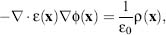
where ε(x) is a spatially varying dielectric coefficient,  (x)is the electrostatic potential
(in units of V), ε0 = 8.854 x 10⁻¹²F/m is the
permittivity of a vacuum, and ρ(x) is the charge density (in units of C/m3)
that generates (x). The dielectric
coefficient ε(x) typically assumes different values inside the solute and in the bulk
solvent to reflect the relative polarizabilities of the two media. For biomolecules in an aqueous
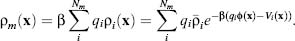
environment, ε is generally given a value of 2-20 inside the solute and a value of 80 in the solvent. Figure 24.1a shows the traditional
definition of ε(x) which includes a jump discontinuity across the molecular
surface while ε(x) changes between the protein and solvent dielectric values.
However, more recent work (Im, Beglov, and Roux, 1998; Grant, Pickup, and Nicholls, 2001; Schnieders et
al., 2007) has proposed smoother definitions for ε(x) to reduce artifacts
arising from the rapidly changing coefficient.
(x)is the electrostatic potential
(in units of V), ε0 = 8.854 x 10⁻¹²F/m is the
permittivity of a vacuum, and ρ(x) is the charge density (in units of C/m3)
that generates (x). The dielectric
coefficient ε(x) typically assumes different values inside the solute and in the bulk
solvent to reflect the relative polarizabilities of the two media. For biomolecules in an aqueous
environment, ε is generally given a value of 2-20 inside the solute and a value of 80 in the solvent. Figure 24.1a shows the traditional
definition of ε(x) which includes a jump discontinuity across the molecular
surface while ε(x) changes between the protein and solvent dielectric values.
However, more recent work (Im, Beglov, and Roux, 1998; Grant, Pickup, and Nicholls, 2001; Schnieders et
al., 2007) has proposed smoother definitions for ε(x) to reduce artifacts
arising from the rapidly changing coefficient.
Likewise, the charge distribution ρ(x) has typically been given a very discontinuous definition, which can pose numerical difficulties for solution of the Poisson equation. In the absence of mobile counterions, ρ(x) is often treated as a collection of Dirac delta functions that model the Nf atomic partial charges of the solute:
(24.2)
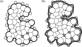
Figure 24.1. Popular definitions of the poisson-Boltzmann equation coefficients. (a) The molecular surface (solid black line )often used to define the dielectric coefficient ε(x). This surface can be constructed by rolling solvent probes (small hatched circles) over the macromolecule (large white spheres). Gray regions show areas outside the atomic volume that are treated as “inside” the molecular surface. (b) The ion-accessible volume is the region outside the solid black line. This volume is defined as the region of space accessible to ion probe spheres (hashed circles).
where qi are the magnitudes of the atomic partial charges (in units of C), and xi are the partial charge positions. The Dirac delta function is a point distribution function with the property ∫f(x)δ(y—x)dx = f (y) and hence has units of m–3.
The PBE is a variant of the Poisson equation where mobile counterion charges are introduced
to the charge distribution function such that ρ(x)= ρf (x) + ρm(x), where ρm(x) denotes the mobile charge distribution. Mean field, or Debye-Huckel,
electrolyte theory describes the distribution of each counterion species i as
ρi(x) = 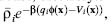 , where
  is the bulk
concentration (in m–3) of species i, β = (kBT)–1 is the inverse thermal
energy, kB is Boltzmann’s constant, T is the temperature, qi (x) is the electrostatic energy of placing a
counterion with charge qi at position x in the potential (x), and Vi(x) is a steric energy
function that prevents mobile charges from entering the interior of the solute. This representation
allows the mobile charge distribution function for Nm counterion species to be written as
is the bulk
concentration (in m–3) of species i, β = (kBT)–1 is the inverse thermal
energy, kB is Boltzmann’s constant, T is the temperature, qi (x) is the electrostatic energy of placing a
counterion with charge qi at position x in the potential (x), and Vi(x) is a steric energy
function that prevents mobile charges from entering the interior of the solute. This representation
allows the mobile charge distribution function for Nm counterion species to be written as
In the case of a 1:1 monovalent ion distribution where the steric functions Vi are equal (e.g., Vi = V), Eq. 24.3 can be simplified to pm(x) = 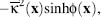 where
where 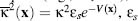 is the dielectric constant of the
bulk solvent, and k is the Debye-Huckel parameter, defined for a general Nm-component electrolyte solution as
is the dielectric constant of the
bulk solvent, and k is the Debye-Huckel parameter, defined for a general Nm-component electrolyte solution as 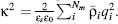 As illustrated in Figure 24.1b, the
function e–βV(x) is usually treated as a
discontinuous characteristic function equal to unity within an ion-accessible volume (typically slightly
larger than the protein volume) and zero otherwise. The PBE for a 1:1 monovalent electrolyte is
therefore
As illustrated in Figure 24.1b, the
function e–βV(x) is usually treated as a
discontinuous characteristic function equal to unity within an ion-accessible volume (typically slightly
larger than the protein volume) and zero otherwise. The PBE for a 1:1 monovalent electrolyte is
therefore
(24.4)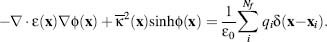
For sufficiently small values of (x), the approximation sinh( (x)) ~ (x) is often applied to this
equation to give the linearized PBE:
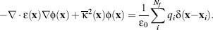
All these equations are solved in conjunction with a Dirichlet boundary condition, which specifies the value of potential at the boundary of some domain. For a sufficiently large domain, this condition is typically zero or some asymptotic form of the solution, such as the Debye-Huckel potential.
The PBE can also be derived from statistical mechanics using a continuum representation of the solvent dielectric properties (Netz and Orland, 2000; Holm, Kekicheff and Podgornik, 2001). While such treatments are too complicated to present here, one important aspect of these derivations is the development of a field theoretic framework for electrostatic interactions with the construction of the PBE as the “saddle point” equation for the potential that minimizes a relevant electrostatic “action” or energy.
Energies
As discussed above, the PBE defines an electrostatic energy that can be derived from physical chemistry arguments (Sharp and Honig, 1990) or field theory saddle point approximations (Netz and Orland, 2000; Holm, Kekicheff and Podgornik, 2001). The free energy is a functional of the electrostatic potential as well as the atomic positions, charges, and radii. For a 1: 1 monovalent electrolyte, this functional has the form
(24.6)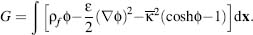
The first term, ∫ρf dx, is the energy of inserting the protein
charges into the electrostatic potential and can be interpreted as the energy of interaction for the
fixed charges. The second term,  represents
electrostatic stresses in the dielectric medium. Finally, the third term includes the effects of the
mobile charge configuration and can be interpreted in terms of the excess osmotic pressure of the
system. The subtraction of unity from the exponential in this term makes this an excess osmotic pressure
and is necessary to cause the energy to vanish in the absence of a potential. Like the PBE, this energy
expression can be linearized (see Eq.
24.5) for sufficiently small by
assuming cosh ( (x)) ~ 1 + (x)2/2. This linearized form of the energy leads to an additional
simplification; Gauss’Law allows the second term to be rewritten as
represents
electrostatic stresses in the dielectric medium. Finally, the third term includes the effects of the
mobile charge configuration and can be interpreted in terms of the excess osmotic pressure of the
system. The subtraction of unity from the exponential in this term makes this an excess osmotic pressure
and is necessary to cause the energy to vanish in the absence of a potential. Like the PBE, this energy
expression can be linearized (see Eq.
24.5) for sufficiently small by
assuming cosh ( (x)) ~ 1 + (x)2/2. This linearized form of the energy leads to an additional
simplification; Gauss’Law allows the second term to be rewritten as 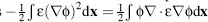 and gives two equivalent free energy expressions
(24.7)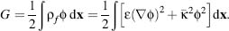
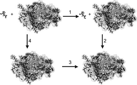
These free energy expressions can be used for a variety of static calculations on biomolecules, including the determination of binding constants, pKas, and solvation energies. These calculations are typically performed from a series of Poisson-Boltzmann energy evaluations that are then analyzed by free energy cycles. Figure 24.2 shows the specific case of pKa calculations, where the energy of protonating a functional group in a biomolecule is calculated in a stepwise fashion by determining the energies of the isolated biomolecule without the functional group, the isolated functional group in its protonated and unprotonated state, the biomolecule with the protonated functional group, and the biomolecules with the unprotonated functional group. These energies are then combined (as shown in Figure 24.2) to give the free energy of protonating the functional group in the biomolecular environment, which can be converted to a pKa value. Similar cycles are used to calculate binding and solvation energies.
Forces
Poisson-Boltzmann calculations have also found an increasingly important role in force evaluation for implicit solvent dynamics simulations. In such simulations, the dynamical trajectory of a solute is calculated without the inclusion of the numerous explicit solvent molecules required for traditional molecular dynamics simulations. Instead, the solvent effects are modeled by stochastic forces applied to the biomolecule to mimic solvent buffeting, damping forces to provide the effect of solvent viscosity, continuum approximations of apolar interactions, and continuum electrostatics calculations (such as PBE) to include the effects of implicit solvent and salt on electrostatic forces in the solute.
Figure 24.2. Titration calculation for a GLU 35 in the active site of hen egg white lysozyme (PDB ID 2LZT). The free energy of protonating GLU 35 (blue ball and stick moiety) in the presence of a biomolecule (cyan object) is calculated by a thermodynamic cycle. Specifically, the free energy of interest ΔG3 is calculated in terms of the other steps in the cycle, ΔG1 the energy of protonating the isolated GLU in solution (related to the “model pKa”), ΔG2 the energy of “binding” the protonated GLU to the lysozyme structure, and ΔG4 the energy of “binding” the unprotonated GLU to the lysozyme structure, such that ΔG3 can be calculated from a thermodynamic cycle as ΔG3 = ΔG1 + G2 – ΔG4. Figure from Reviews in Computational Chemistry, N. Baker. Figure also appears in the Color figure section.
To derive forces from the PBE, we simply differentiate the free energy with As mentioned
previously, a potential , which solves the
PBE, is a saddle point of G, that is, ∂G/∂ = 0. Therefore, the force Fi on atom i can be written solely in terms of variations in the coefficients with
respect to atomic displacements ∂ yi
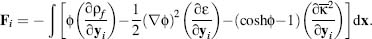
The terms of the integrand in this force expression have the same interpretation as for the
free energy. The first term is the force density for atomic displacements in the potential , the second is the dielectric boundary
pressure on atom i, and the third is osmotic pressure on atom i.
The mechanics of evaluating atomic forces from Eq. 24.8 have been discussed in detail in the literature (Gilson et al., 1993; Im, Beglov and Roux, 1998). These authors present excellent reviews of this topic, including the effects of discontinuities in the PBE coefficients ε and k2 on the methods for force evaluation and the accuracy of the numerical results.
NUMERICAL SOLUTION OF THE POISSON-BOLTZMANN EQUATION
Very few analytical solutions of the Poisson-Boltzmann equation exist for realistic biomolecular geometries and charge distributions. Therefore, this equation is usually solved numerically by a variety of computational methods. These methods typically rely on a discretization to project the continuous solution down onto a finite-dimensional set of basis functions. In the case of the linearized PBE (Eq. 24.5), the resulting equations are the usual linear matrix-vector equation, which can be solved directly. However, the nonlinear equations obtained from the full PBE require more specialized techniques, such as Newton methods, to determine the solution to the discretized algebraic Specifically, Newton methods start with an initial solution guess and iteratively improve this guess by solving related linear equations for corrections to the current solution. Newton methods, as well as other popular methods for solution of nonlinear equations, have been reviewed by Holst and Saied (1995).
Multilevel Finite Difference and Finite Element Methods
Some of the most popular discretization techniques employ Cartesian meshes to subdivide the domain in which the Poisson-Boltzmann equation is to be solved. Of these, the finite difference method has been at the forefront of PBE solvers. In its most general form, the finite difference method solves the PBE on a nonuniform Cartesian mesh, as shown in Figure 24.3a for a two-dimensional domain. While Cartesian meshes offer relatively simple problem setup, they provide little control over how unknowns are placed in the solution domain. Specifically, as shown by Figure 24.3a, the Cartesian nature of the mesh makes it impossible to locally increase the accuracy of the solution in a specific region without increasing the number of unknowns across the entire grid.
Differential operators for problems discretized by finite difference methods are typically approximated using Taylor expansions. For example, a discretized one-dimensional Laplacian operator has the form
(24.9)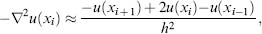
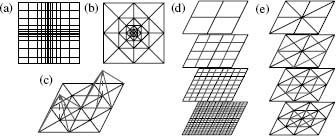
Figure 24.3. Meshes and hierarchies used in Poisson–Boltzmann solvers. (a) Cartesian mesh suitable for finite difference calculations; nonuniform mesh spacing can be used to provide a limited degree of adaptivity. (b) Finite element mesh exhibiting adaptive refinement. (c) Examples of typical piecewise linear basis functions used to construct the solution in finite element methods. (d) The multilevel hierarchy used to solve the PBE for a finite difference discretization; red lines denote the additional unknowns added at each level of the hierarchy. (e) The multilevel hierarchy used to solve the PBE for a finite element discretization; red lines denote simplex the subdivisions used to introduce additional unknowns at each level of the hierarchy. Figure also appears in the Color figure section.
where xj denotes the grid point coordinates and h is the mesh spacing. Given vectors u and f representing the values of the solution and source terms at the grid points, it is straightforward to develop a matrix form of the problem Au = f, where A is a sparse symmetric matrix with 2 on the main diagonal, –1 on the first off-diagonal elements, and 0 elsewhere in the matrix. Discretization of the differential operator for the PBE yields a matrix with a similar sparse symmetric structure, but more nonzeros per row.
Unlike finite difference methods, adaptive finite element discretizations offer the ability to place computational effort on specific regions of the problem domain. Finite element meshes (see Figure 24.3b) are composed of simplices that are joined at edges and vertices. The solution is constructed from piecewise polynomial basis functions (Figure 24.3c) that are associated with mesh vertices and typically are nonzero only over a small set of neighboring simplices. Solution accuracy can be increased in specific areas by locally increasing the number of vertices through simplex refinement (subdivision). As shown in Figure 24.3b, the number of unknowns (vertices) is generally increased only in the immediate vicinity of the simplex refinement and not throughout the entire problem domain as in finite difference methods. This ability to locally increase the solution resolution is called “adaptivity” and is the major strength of finite element methods applied to the PBE (Holst et al., 2000; Baker, Holst, and Wang, 2000; Baker, et al., 2001a).
Typically, the algebraic system is assembled using a Galerkin discretization, where a “weak” form of the PBE is imposed for each basis function in the system. Specifically, the original differential form of the PBE is transformed by integration with a basis function v to give an integral equation
The algebraic system is implicitly assembled by representing the solution as a linear
combination of finite element basis functions  and imposing the weak PBE (Eq. 24.10) using every basis function ψj as test
functions. As with the finite difference method, this discretization scheme leads to sparse symmetric
matrices with a small number of nonzero entries in each row.
and imposing the weak PBE (Eq. 24.10) using every basis function ψj as test
functions. As with the finite difference method, this discretization scheme leads to sparse symmetric
matrices with a small number of nonzero entries in each row.
Multilevel solvers, in conjunction with the Newton methods described above, have been shown to provide most efficient solution of the algebraic equations obtained by discretization of the PBE with either finite difference or finite element techniques. Most sizable algebraic equations are solved by iterative methods that repeatedly apply a set of operations to improve an initial guess until a solution of the desired accuracy is reached. However, the speed of traditional iterative methods has been limited by their inability to quickly reduce low-frequency (long-range) error in the solution. Multilevel methods overcome this problem by projecting the discretized system onto meshes (or grids) at multiple resolutions (see Figure 24.3). The advantage of this multiscale representation is that the slowly converging low-frequency components of the solution on the finest mesh are quickly resolved on coarser levels of the system. This gives rise to a multilevel solver algorithm, where the algebraic system is solved directly on the coarsest level and then used to accelerate solutions on finer levels of the mesh.
As shown in Figure 24.3, the assembly of the multiscale representation, or “multilevel hierarchy,” depends on the method used to discretize the PBE. For finite difference types of methods, the nature of the grid lends itself to the assembly of a hierarchy with little additional work. In the case of adaptive finite element discretizations, the most natural multiscale representation is constructed by refinement of an initial mesh that typically constitutes the coarsest level of the hierarchy.
Boundary Element Solvers
The finite difference and finite element methods described above have substantial computational requirements for large systems, due in part to the storage and computation of data for points that are distributed throughout the volume of the system. In principle, boundary element methods have the advantage of limiting the analysis to the molecular surfaces, so that substantially fewer grid points need be considered; the number of unknowns is therefore greatly reduced in the corresponding algebraic system. Boundary element methods have their own limitations, however. First, because of their physical formulation, they are limited to solving the linearized PBE. Second, the potential advantages in numerical efficiency were lost in early applications due to the use of Gaussian elimination in the treatment of the dense matrix in the algebraic system; storage and computational operations were scaled with the square and the cube of the number of boundary nodes, respectively. Fast multipole methods (FMM) offer a way to offset these inefficiencies by introducing reduced, collective descriptions of contiguous elements on distant boundaries. A recent implementation of FMM has achieved linear scaling in the number of boundary nodes, and additional efficiencies have been achieved by careful placement of nodes and boundary elements (see Lu et al., 2006; Lu and McCammon, 2007). Continuing efforts along these lines should be helpful in reducing the cost of electrostatic calculations in the context of high-throughput proteomics studies and simulations of interacting protein molecules with frequent updating of the electrostatic forces.
APPLICATIONS
Applications of biomolecular electrostatics methods can be found in many different areas of computational biophysics and structural bioinformatics. Note that, in all of these applications, electrostatics is but one component of the overall system that also includes nonpolar effects, conformational energetics, and entropic changes. The scope of our discussion will necessarily be limited to electrostatics; however, interested readers should refer to work by others for a more detailed description of binding phenomena (Kollman et al., 2000; Swanson, Henchman and McCammon, 2004; Woo and Roux, 2005). The following sections highlight some of the major applications of these methods to biomolecular thermodynamics, kinetics, and bioinformatics.
Thermodynamics
The application of electrostatics methods to thermodynamic processes in biophysics necessarily involves the calculation of free energies, as outlined in Section “Energies.” In general, such applications are interested in changes in energy associated with a particular biomolecular transformation such as protonation, ligand binding, folding, or other conformational changes. There are far too many examples of these applications to discuss in detail, however, a few particular examples illustrate some of the basic principles.
As mentioned above (Section “Energies”) and illustrated in Figure 24.2, electrostatics methods are commonly used to evaluate pKa values for amino acid and nucleic acid residues in the context of specific biomolecular structures (Bashford and Karplus, 1990; Yang et al., 1993; Antosiewicz, McCammon, and Gilson, 1996). Such applications not only provide important insight into biomolecular function but also serve as a critical test for the accuracy of continuum electrostatics methods. As a result of continual comparison between calculated and experimental pKa values, new methods for pKa calculations have evolved to include important contributions from local hydrogen bonding (Nielsen and Vriend, 2001) and environment (Li, Robertson and Jensen, 2005), conformational flexibility (Georgescu et al., 2002), and large-scale rearrangement in biomolecular structures (Whitten and García-Moreno, 2005).
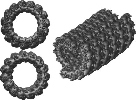
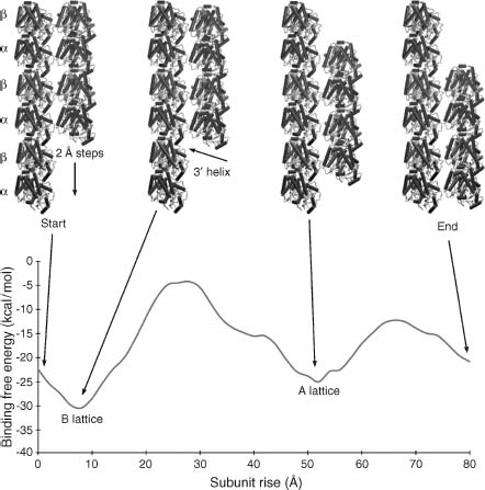
Biomolecular electrostatics can also provide insight into macromolecular assembly and function through analysis of protein-protein interactions as well as larger-scale assemblages. In particular, electrostatics calculations on macromolecular complexes demonstrate some of the demands for scalability and efficiency in electrostatics software. Some examples of such applications include analysis of microtubule electrostatics (Baker et al., 2001b) and proto-filament assembly (Sept, Baker and McCammon, 2003) (see Figure 24.4), viral capsid electrostatics (Zhang et al., 2004; Konecny et al., 2006), and ribosome electrostatic properties (Baker et al., 2001b; Trylska et al., 2004; Trylska et al., 2005). Other work on molecular assemblages investigates electrostatic properties of lipid bilayers. An excellent example of such membrane studies is provided in work by Murray and Honig (2002). This work focused on C2 domains, a large group of sequentially varied but structurally conserved modules that targets the binding of proteins involved in signal transduction, membrane trafficking and fusion, and other cellular activities. Murray and Honig demonstrated that the targeting of C2 modules is determined in large part by electrostatics. For example, the membrane binding faces of C2 modules from protein kinase C become positively charged when the modules coordinate calciumions, causing a calcium-triggered binding to negatively charged patches of membrane. By contrast, the corresponding face of C2 modules from cytosolic phospholipase A2 switch from a negative to neutral character upon coordination of calcium ions; the binding of these ions triggers binding to neutral membranes by reducing the unfavorable free energy of dehydration of the charged face upon contact with the membrane. Murray and Honig show how these principles can be used to rationalize or predict the binding properties of other C2 modules, including ones whose structures are based on homology modeling.
Figure 24.4. Microtubule electrostatics. (a) Electrostatic properties of a 1.2 million atom 400 × 300 × 300Å microtubule fragment illustrating the current state of the art for continuum electrostatics calculations. The potential was calculated using APBS to solve the PBE at 150mM ionic strength; more details are available in Baker et al. (2001b). (b) Apotential of mean force, calculated using continuum electrostatics and a simple nonpolar function, describing microtubule protofilament assembly; more details are available in Sept, Baker and McCammon (2003). Part B is from Sept, Baker, and McCammon. Figure also appears in the Color figure section.
Kinetics
A very wide variety of kinetic processes involving proteins are governed in large part by electrostatic interactions. These include the electrostatically steered binding of substrates or macromolecules to proteins and the association of proteins with membranes. Faster and more accurate methods for calculating electrostatic forces are therefore critical to the computational analysis of such processes. The actual dynamics can be simulated in various ways. The Brownian dynamics method, mentioned earlier, treats the diffusing solute molecules explicitly as structured objects with one or more centers of interaction. Several reviews of work in this area are available (Elcock, Sept, and McCammon, 2001; Gabdoulline and Wade, 2002). It has been possible with such calculations to replicate the experimentally observed rates of association of such protein pairs as barnase-barstar and fasciculin 2-acetylcholinesterase, including the variations in the rates as functions of ionic strength and protein mutagenesis. Similar calculations, by Sept and McCammon (2001), have provided a basis for understanding the nucleation and growth of polar actin filaments.
Brownian dynamics has been employed recently in a ground breaking simulation of the diffusion of 1000 interacting protein molecules (McGuffee and Elcock, 2006). Here, the electrostatic interactions among the proteins were treated by use of effective charges, whose magnitudes were calibrated by Poisson-Boltzmann calculations. When the diffusing solutes are small enough to be treated as structureless, they can be represented implicitly as a concentration or density distribution. Their dynamics can then be described by solution of the diffusion or Smoluchowski equation, instead of stepping the solutes through time individually as in Brownian dynamics. Recent progress in this approach allows simulation of the time-dependent diffusion and reaction of solutes in this continuum representation, including the effects of electrostatics (Cheng et al., 2007). As discussed in a recent review by Stein, Gabdoulline and Wade (2007), algorithmic advances in simulation methodology are enabling investigation of biomolecular encounter kinetics at the scales of biochemical networks and systems.
Electrostatic Comparisons
Effort has also been made to pursue more “informatics”-based approaches to the interpretation of electrostatic properties. Much of this work includes identification of functionally relevant residues in biomolecules by looking at electrostatic destabilization of conserved residues (Elcock, 2001), characteristics of titration curves (Ondrechen, Clifton and Ringe, 2001), or localization of charged groups (Zhu and Karlin, 1996). Other research has focused on comparisons of electrostatic potentials including global analyses of potential both in three-dimensional space over the entire biomolecular structure and at localized regions such as active sites (Blomberg et al., 1999; Livesay et al., 2003; Livesay and La, 2005; Saito, Go, and Shirai, 2006; Zhang et al., 2006, in the reference section). Characterization of electrostatic properties of biomolecules has provided insight into a variety of biomolecular properties, including functional similarities, ligand binding specificities, as well as protein-protein and protein-DNA binding sites. Potential uses for these methods are likely to grow with increases in both biomolecular structural data and information about biomolecular interaction networks. With such growth, tools to facilitate the analysis of electrostatic properties across thousands of biomolecular structures will continue to be very important.
FUTURE DIRECTIONS
In the future, it should be possible to apply continuum electrostatics methods to help determine and investigate macromolecular interactions within increasingly larger assemblages and, eventually, at the cellular scale. Some future research is likely to focus on the computational evaluation of the thermodynamics and kinetics of biomolecular interactions, moving beyond pairs of interacting proteins to biochemical networks of proteins, nucleic acids, metabolites, and many other biochemical species. New computational methods suitable for much larger systems will allow for studies the structure and dynamics of such macromolecular assemblages as ribosomes and elongation factors; the machinery of DNA replication, repair, and transcription; the nuclear pore complex; and a host of other cellular components. In addition, research continues to improve the ability to use electrostatics to screen and compare biomolecular structures for specific function or similarity to other molecules. Finally, the computational biophysics community will continue to improve implicit solvent models to provide increasing accuracy and reliability in describing biomolecular systems with diverse geometries and charge densities. For all of these tasks, high-throughput continuum electrostatics methods will facilitate the development of computational proteomics to determine the network of biomolecular reactions in living organisms.
TABLE 24.1. Some of the Software that Implements the Concepts Described in this Chapter
| Program | Description | URL |
| DelPhi | Solves the PBE using highly optimized finite difference methods. | http://trantor.bioc.colum bia.edu/delphi/ |
| APBS | Solves the PBE using parallel multigrid and parallel adaptive finite element methods. | http://apbs.sf.net/ |
| MEAD | Solves the PBE using finite difference methods and determines pKa values while incorporating conformational flexibility of the macromolecule. | http://www.scripps.edu/bash ford/ |
| UHBD | Solves the PBE using finite difference methods, calculates binding and solvation energies, determines pKas, and performs Brownian dynamics simulations. | http://mccammon.ucsd.edu/uhbd.html |
| AMBER | In addition to providing explicit solvent simulation tools, this package implements generalized Born and PBE-based implicit solvent methods in both dynamics and free energy evaluation simulations. | http://amber.scripps.edu |
| CHARMM | In addition to providing explicit solvent simulation tools, this package implements generalized Born and PBE-based implicit solvent methods in both dynamics and free energy evaluation simulations. | http://charmm.org/ |
| Qnifft | Poisson–Boltzmann finite difference solver developed by the Sharp lab. | http://crystal.med.upenn.edu/software.html |
ACKNOWLEDGMENTS
Support for this work was provided in part by HHMI and the National Biomedical Computation Resource. Additional support has been provided by grants to N.A.B. from NIH and the Sloan Foundation and by grants to J.A.M. from NIH, NSF, the NSF Supercomputer Centers, the Center for Theoretical Biological Physics, and Accelrys.