Structural Bioinformatics

PREDICTION OF PROTEIN STRUCTURE IN 1D: SECONDARY STRUCTURE, MEMBRANE REGIONS, AND SOLVENT ACCESSIBILITY

Burkhard Rost

INTRODUCTION

No General Prediction of 3D Structure from Sequence, Yet

The hypothesis that the 3D structure¹ of a protein (the fold) is uniquely determined by the specificity of the sequence has been verified for many proteins (Anfinsen, 1973). While particular proteins (chaperones) often play an important role in folding (Ellis, Dobson, and Hartl, 1998), it is still generally assumed that the final structure is at the free-energy minimum (Dobson and Karplus, 1999). Thus, all information about the native structure of a protein is coded in the amino acid sequence and its native solution environment. Can we decipher the code; that is, can we predict 3D structure from sequence? In principle, the code could by deciphered from physicochemical principles (Levitt and Warshel, 1975; Hagler and Honig, 1978). In practice, the inaccuracy in experimentally determining the basic parameters and the limited computing resources prevent prediction of protein structure from first principles (van Gunsteren, 1993). Hence, the only successful structure prediction tools are knowledge-based, using a combination of statistical theory and empirical rules. The field of protein structure prediction has advanced significantly over the past 15 years (see Chapter 28) with improved methods (Kryshtafovych et al., 2005; Moult et al., 2005). However, possibly the most important change was the growth of the PDB (Berman et al., 2002) that increases the odds of finding local 3D matches to build comparative models (Chance et al., 2004). We can, however, still not predict structure from sequence reliably without finding related sequences of known structure in the databases (Moult et al., 2005).

Structure Prediction in 1D has become Increasingly Accurate and Important

An extreme simplification of the prediction problem is to project 3D structure onto strings of structural assignments. For example, we can assign a secondary structure state, marked by one symbol, for each residue, or we can assign a number for the accessibility of that residue. Such strings of per-residue assignments are essentially one-dimensional (1D). In fact, arguably the most surprising improvements in bioinformatics over the last decade may have been achieved by methods predicting protein structure in 1D. The key to this breakthrough was the wealth of evolutionary information contained in ever-growing databases. Moreover, prediction accuracy continues to rise (Rost, 2001). This success is crucial for target selection in structural genomics (Liu et al., 2004), for using structure prediction to get clues about function (Rost et al., 2003; Ofran et al., 2005), and for using simplified predictions for more sensitive database searches and predictions of higher dimensional aspects of protein structure (see below).

Apologies to Developers!

This brief synopsis of methods predicting protein structure in 1D has no chance of being fair to all developing methods for 1D protein structure prediction. Even a MEDLINE search restricted to “secondary structure prediction” revealed more than 100 publications over the last year. Consequently, the review will be somehow unfair to the majority of developers. Instead, the focus lies on the small subset of most accurate or most widely used methods.

METHODS

Secondary Structure Prediction Methods

Basic Concept. The principal idea underlying most secondary structure prediction methods is the fact that segments of consecutive residues have preferences for certain secondary structure states (Brändén and Tooze, 1991; Rost, 1996). Thus, the prediction problem becomes a pattern classification problem tractable by pattern recognition algorithms. The goal is to predict whether a residue is in a helix, in a strand, or in none of the two (no regular secondary structure, often referred to as the “coil” or “loop” state). The first-generation prediction methods in the 1960s and ’70s were all based on single amino acid propensities (Chou and Fasman, 1974; Robson, 1976; Garnier, Osguthorpe, and Robson, 1978; Schulz and Schirmer, 1979; Fasman, 1989). Basically, these methods compiled the probability of a particular amino acid for a particular secondary structure state. The second-generation methods dominated the scene until the early 1990s; they extended the principal concept to compiling propensities for segments of adjacent residues; that is, taking the local environment of the residues into consideration. Typically methods used segments of 3-51 adjacent residues (Nishikawa and Ooi, 1982; Nishikawa and Ooi, 1986; Deleage and Roux, 1987; Biou et al., 1988; Bohr et al., 1988; Gascuel and Golmard, 1988; Levin and Garnier, 1988; Qian and Sejnowski, 1988; Garnier and Robson, 1989). Basically, any imaginable theoretical algorithm had been applied to the problem of predicting secondary structure from sequence: physicochemical principles, rule-based devices, expert systems, graph theory, linear and multilinear statistics, nearest-neighbor algorithms, molecular dynamics, and neural networks (Schulz and Schirmer, 1979; Fasman, 1989; Rost and Sander, 1996; Rost and Sander, 2000). However, it seemed that prediction accuracy stalled at levels around 60% of all residues correctly predicted in either of the three states helix, strand, or other. It was argued that the limited accuracy resulted from the fact that all methods used only information local in sequence (input: about 3-51 consecutive residues). Local information was estimated to account for roughly 65% of the secondary structure formation. Two additional problems were common to most methods developed from 1957 to 1993. First, predicted secondary structure segments were, on average, only half as long as observed segments. Historically, this problem was solved for the first time through a particular combination of neural networks (Rost and Sander, 1992; Rost and Sander, 1993). Second, strands were predicted at levels of accuracy only slightly superior to random predictions. Again, the argument for this deficiency was that the hydrogen bonds determining the formation of sheets (note: paired strands form a sheet) are less local in sequence than the bonds responsible for helices (Chapter 19). Again, this problem was first solved through neural networks (Rost and Sander, 1992; Rost et al., 1993). The solution was rather simple: we realized that about 20% of the correctly predicted residues were in strands, about 30% in helices, and about 50% in nonregular secondary structure. These values are similar to the percentage of the respective classes in proteins. This observation prompted us to simply bias the database used for training neural networks by presenting each class equally often. The result was a prediction well balanced between the three classes, that is, about 60% of the strand residues were correctly predicted. In practice, this was an important advance. However, it also cast an important spotlight onto the explanation that secondary structure formation is partially determined by nonlocal interactions. Clearly, sheets are nonlocal structures. Nevertheless, the preferences for a segment to form a strand or a helix appear similarly strong because both can be predicted at similar levels of accuracy designing the appropriate prediction method (Rost and Sander, 1993; Rost and Sander, 1994a; Rost, 1996).

Evolutionary Information Key to Significantly Improved Predictions. On the one hand, about 67 out of 100 residues can be exchanged in a protein without changing structure (Rost, 1999). On the other hand, exchanges of very few residues often destabilize a protein structure. The explanation for this ostensible contradiction is simple: evolution has realized the unlikely by exploring all neutral mutations that do not prevent structure formation. Thus, the residue exchange patterns extracted from an aligned protein family are highly indicative of specific structural details. This also implies that a profile of a few consecutive residues taken from alignments implicitly contains nonlocal information. The source of this information is that evolutionary selection acts on a 3D object (the protein) rather than on an abstracted 1D construct (the sequence). Early on, it was realized that this information could improve predictions (Dickerson, Timkovich, and Almassy, 1976; Maxfield and Scheraga, 1979; Zvelebil et al., 1987). However, the breakthrough of the third-generation methods to levels above 70% accuracy required a combination of larger databases with more advanced algorithms (Rost et al., 1993; Rost and Sander, 2000). It was also recognized very early on that information from the position-specific evolutionary exchange profile of a particular protein family facilitates discovering more distant members of that family (Dickerson, Timkovich, and Almassy, 1976). Automatic database search methods successfully used position-specific profiles for searching (Barton, 1996). However, the breakthrough to large-scale routine searches has been achieved by the development of PSI-BLAST (Altschul et al., 1997) and hidden Markov models (HMMs) (Eddy, 1998; Karplus, Barrett, and Hughey, 1998). Since the improvement of secondary structure prediction relies significantly on the information content of the family profile used, today’s larger databases and better search techniques resulted in pushing prediction accuracy even higher. The current top-of-the-line secondary structure prediction methods are all based on extended profiles (Rost, 2001; Przybylski and Rost, 2002).

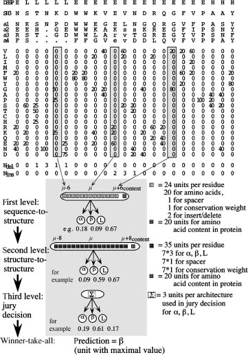
Key Players. PHD was the program that surpassed the level of 70% accuracy first (Rost and Sander, 1993; Rost and Sander, 1994). It uses a system of neural networks to achieve a performance well balanced between all secondary structure classes (Figure 29.1). Although still widely used, PHD is no longer the most accurate method (Rost and Eyrich, 2001; Przybylski and Rost, 2002). David Jones pioneered using automated, iterative PSI-BLAST searches (Jones, 1999b). The most important step climbed by the resulting method PSIPRED has been the detailed strategy to avoid polluting the profile through unrelated proteins. To avoid this trap, the database searched has to be filtered first (Jones, 1999). Other than the advanced use of PSI-BLAST, PSIPRED achieves its success through a neural network system similar to that implemented in PHD. At the CASP meeting at which David Jones introduced PSIPRED, Kevin Karplus and colleagues presented their prediction method (SAM-T99sec/SAM-T04) finding more diverged profiles through HMMs (Karplus et al., 1999). The most important prediction method used by SAM-T99sec is a simple neural network with two layers of hidden units. However, the major strength of the method appears to be the quality of the alignment used. Some recent methods improve accuracy significantly not through more divergent profiles but through the particular algorithm; examples are the SSpro series of programs, the latest is SSpro4 (Pollastri et al., 2002a; Pollastri et al., 2002b), and Porter (Pollastri and McLysaght, 2005). The principal idea is to overcome the limitations of feed-forward neural networks with an input window of relative small and fixed size with bidirectional recurrent neural networks (BRNN) capable of taking the entire protein chain as input (Pollastri et al., 2006). The latest implementation SSpro4 uses this concept in combination with advanced PSI-BLAST profiles to become one of the best existing methods. Porter (Pollastri and McLysaght, 2005) goes beyond SSpro4 by also using details in the alignment more cleverly and by combining a variety of different networks. Porter may be the most accurate existing method for the prediction of secondary structure. Another method that reaches high accuracy is SABLE2 (Adamczak, Porollo, and Meller, 2004; Adamczak, Porollo, and Meller, 2005) that combines the prediction of secondary structure and solvent accessibility; PROFsec and PROFacc realize the same idea in a similar way (Rost, 2005). One recent method reached very high levels of prediction accuracy without paying for this achievement by complexity: YASPIN combines HMMs with neural networks in a very simple and efficient way (Lin et al., 2005). Quite a different route toward secondary structure prediction is taken by the HMMSTR/I-sites programs (Bystroff et al., 2000).

Specialized Methods: Coiled Coil Predictions. A coiled coil is abundle of several helices assuming a side-chain packing geometry often referred to as “knobs-into-holes” (Crick, 1953). The “knobs” are the side chains of one helix that pack into the hole created by four side chains surrounding the facing helix. This supercoil slightly alters the helix periodicity from 3.6 to 3.5 and results in the coiled-coil-specific symmetry in which every seventh residue occupies a similar position on the helix surface. The first and fourth of the seven residues are typically hydrophobic, the other four hydrophilic, frequently exposing the helix to solvent. These specific sequence features are at the base of accurate predictions for coiled coil helices (Lupas, 1996,1997). The most widely used program is COILS that is based on amino acid preferences compiled for the few coiled coil proteins that were known at high resolution a decade ago (Lupas et al., 1991). The program detects coiled coil preferences in windows of 14, 21, and 28 residues. The longer the window the better the distinction between proteins that have coiled coil regions and those that do not (Lupas, 1996). If we know the precise location of the coiled coil regions and the multimeric state, we can predict 3D structure for coiled coil regions at levels of accuracy that resemble experimentally determined structures (below 2.5 Å; Nilges and Brunger, 1993; O’Donoghue and Nilges, 1997). O’Donoghue and Nilges used the experimentally known boundaries of the coiled coil regions and their known multimeric state for prediction. It reains to be tested how sensitive that 3D prediction is with respect to errors in predicting the coiled coil regions. Recently, Wolf and coworkers developed a method to predict the multimeric state of a coiled coil region (Wolf, Kim, and Berger, 1997; Newman, Wolf, and Kim, 2000). When labeling all likely coiled coil proteins in entire proteomes, we found that about 8-10% of all eukaryotic proteins and 2-10% of all proteins in archaebacteria and prokaryotes contain at least one coiled coil region (Liu and Rost, 2001).

Figure 29.1. Neural network system for secondary structure prediction (PHDsec). From the multiple alignment (here guide sequence SH3 plus four other proteins a1–a4; note that lower case letters indicate deletions in the aligned sequence), a profile of amino acid occurrences is compiled. To the resulting 20 values at one particular position m in the protein (one column), three values are added: the number of deletions and insertions, as well as the conservation weight (CW). Thirteen adjacent columns are used as input. The whole network system for secondary structure prediction consists of three layers: two network layers and one layer averaging over independently trained networks.

Other Alphabets. Most secondary structure prediction methods focus on the standard DSSP alphabet of eight states. Many groups have tried to directly predict all eight states and have found that this approach did not bear fruit, possibly because this detailed separation is not supported by data, or more importantly is not conserved in evolution. In fact, we possibly should define the goals of simplifying structure prediction exactly by what is evolutionarily conserved (Rost, Sander, and Schneider, 1994; Zemla et al., 1999). This is exactly what Kevin Karplus and colleagues realized when sampling the space of local alphabets to identify those that are most conserved in evolution and to develop methods that predict exactly these alphabets (Karchin, Cline, and Karplus, 2004). The concept is successful. So far it has remained an exceptional case possibly only because the approach has remained so unique that very few groups have worked on ways of how to use the information predicted by such methods directly.

Solvent Accessibility Prediction Methods

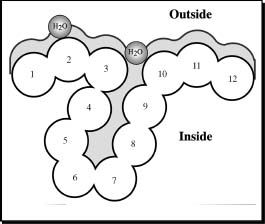
Basic Concept. It has long been argued that if the segments of secondary structure could be accurately predicted, the 3D structure could be predicted by simply trying different arrangements of the segments in space (Mumenthaler and Braun, 1995; Cohen and Presnell, 1996). One criterion for assessing each arrangement could be to use predictions of residue solvent accessibility (Lee and Richards, 1971; Chothia, 1976; Connolly, 1983). The principal goal is to predict the extent to which a residue embedded in a protein structure is accessible to solvent. Solvent accessibility can be described in several ways (Lee and Richards, 1971; Chothia, 1976; Connolly, 1983). The most detailed fast method compiles solvent accessibility by estimating the volume of a residue embedded in a structure that is exposed to solvent (Figure 29.2; this method was developed by Connolly (1983) and later implemented in DSSP (Kabsch and Sander, 1983)). Different residues have a different possible accessible area. The most extreme simplification for accessibility accounts for this by normalizing (dividing observed value by maximally possible value) to a two-state description distinguishing between residues that are buried (relative solvent accessibility less than 16%) and exposed (relative solvent accessibility ≥16%). The precise choice of the threshold is not well defined (Hubbard and Blundell, 1987; Rost and Sander, 1994b). The classical method to predict accessibility is to assign either of the two states, buried or exposed, according to residue hydrophobicity, that is, very hydrophobic stretches are predicted to be buried (Kyte and Doolittle, 1982; Sweet and Eisenberg, 1983). However, more advanced methods have been shown to be superior to simple hydrophobicity analyses (Holbrook, Muskal, and Kim, 1990; Mucchielli-Giorgi, Hazout, and Tuffery, 1999; Carugo, 2000; Li and Pan, 2001; Naderi-Manesh et al., 2001). Typically, these methods use similar ways of compiling propensities of single residues or segments of residues to be solvent accessible, as secondary structure prediction methods. For particular applications, such as using predicted solvent accessibility to predict glycosylation sites, it seems beneficial to train neural networks on different definitions of accessibility (Hansen et al., 1998; Gupta et al., 1999). In particular, Hansen et al. (1998) realized alternative compilations by changing the size of the water molecule used in DSSP (Figure 29.2). In contrast to the situation for secondary structure, most of the information needed to predict accessibility is contained in the preference of single residues (Rost and Sander, 1994). Nevertheless, using windows of adjacent residues also improves solvent accessibility prediction significantly (Rost and Sander, 1994; Thompson and Goldstein, 1996).

Figure 29.2. Measure accessibility. Residue solvent accessibility is usually measured by rolling a spherical water molecule over a protein surface and summing the area that can be accessed by this molecule on each residue (typical values range from 0 to 300Å²). To allow comparisons between the accessibility of long extended and spherical amino acids, typically relative values are compiled (actual area as percentage of maximally accessible area).Amore simplified description distinguishes two states: buried (here residues numbered 1–3 and 10–12) and exposed (here residues 4–9) residues. Since the packing density of native proteins resembles that of crystals, values for solvent accessibility provide upper and lower limits to the number of possible inter-residue contacts.

Evolutionary Information Improves Accessibility Prediction. Solvent accessibility at each position of the protein structure is evolutionarily conserved within sequence families. This fact has been used to develop methods for predicting accessibility using multiple alignment information (Rost, 1994; Thompson and Goldstein, 1996; Cuff and Barton, 2000). The two-state (buried, exposed) prediction accuracy is above 75%, that is, more than four percentage points higher than for methods not using alignment information. Predictions of solvent accessibility have also been used successfully for prediction-based threading, as a second criterion toward 3D prediction, by packing secondary structure segments according to upper and lower bounds provided by accessibility predictions, and as a basis for predicting functional sites (Rost and O’Donoghue, 1997).

Available Key Players. Possibly, the exclusion of methods predicting solvent accessibility from the CASP meetings (see Section “Practical Aspects”) slowed down the progress of the field. In particular, few of the methods developed are readily available through public servers. Prominent exceptions are the solvent accessibility predictions by PHD (Rost and Sander, 1994b) and PROFphd (Rost, 2005) available through the PredictProtein server (Rost, Yachdav, and Liu, 2004; Rost, 1996). Both use systems of neural networks with alignment information. The improvement of PROFphd over PHD was achieved by (1) training the neural networks only on high-resolution structures and by (2) using predicted secondary structure as additional input (Rost, 2001; Rost, 2005). Technically, both PROFphd and PHD are the only available methods predicting real values for relative solvent accessibility on a grid of 0, 1, 4, 9, 16, 25, 36, 49, 64, 81 (percentage relative accessibility). Another method that improved prediction accuracy considerably over older programs is embedded in the JPred2 server (Cuff and Barton, 2000). It uses PSI-BLAST profiles as input to neural networks predicting accessibility in two states (buried/exposed). FKNNacc is based on the identification of related local stretches (k-fuzzy nearest-neighbor methods) (Sim, Kim, and Lee, 2005). More recently several methods have combined the prediction of secondary structure and solvent accessibility; for examples, PROFacc, SABLE2 (Adamczak, Porollo, and Meller, 2004), and ACCpro4 (analogue of SSpro4) (Pollastri et al., 2002a; 2002b).

Related Task: Prediction of Ooi/Coordination Number. The prediction of the residue coordination or Ooi number (Nishikawa and Ooi, 1986b) is directly related to that of the solvent accessibility. This number estimates how many residues surround a particular residue in a sphere. Thereby, the Ooi number provides two boundaries: one for the number of internal bounds and the other for the degree of accessibility to solvent. Several of the recent methods that target the prediction of the Ooi number are based on neural networks (Fariselli et al., 2001; Pollastri et al., 2002a; Pollastri et al., 2002b). A related method simply estimated the contact density based on inter-residue contact predictions succeeded in predicting folding rates (Punta and Rost, 2005). Thus suggesting that the direct relationship between residue coordination and solvent accessibility can also be used to make inferences about the protein folding rates.

Transmembrane Region Prediction Methods

The Task. Even in the optimistic scenario that in the near future most protein structures will be experimentally determined, one class of proteins will still represent a challenge for experimental determination of 3D structure: transmembrane proteins. The major obstacle with these proteins is that they do not crystallize and are hardly tractable by NMR spectroscopy. Consequently, for this class of proteins structure prediction methods are needed even more than for globular water-soluble proteins. Fortunately, the prediction task is simplified by strong environmental constraints on transmembrane proteins: the lipid bilayer of the membrane reduces the degrees of freedom making the prediction almost a 2D problem (Taylor, Jones, and Green, 1994; Bowie, 2005). Two major classes of integral membrane proteins are known: the first insert transmembrane helices (TMH) into the lipid bilayer (Figure 29.3) and the second form pores by transmembrane beta-strand barrels (TMB) (von Heijne, 1996; Seshadri et al., 1998; Buchanan, 1999). While predicting transmembrane helices is simpler than predicting globular helices, there is ample evidence that prediction accuracy has been significantly overestimated (Möller, Croning, and Apweiler, 2001; Chen, Kernytsky, and Rost, 2002).

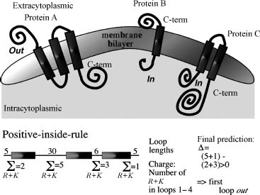
Basic Concept. We can use a number of observations that constrain the problem of predicting membrane helices. (1) TM helices are predominantly apolar and between 12 and 35 residues long (Chen and Rost, 2002). (2) Globular regions between membrane helices are typically shorter than 60 residues (Wallin and von Heijne, 1998; Liu and Rost, 2001). (3) Most TMH proteins have a specific distribution of the positively charged amino acids arginine and lysine, coined the positive-inside rule by Gunnar von Heijne (von Heijne, 1986; von Heijne, 1989). Connecting loop regions at the inside of the membrane have more positive charges than loop regions at the outside (Figure 29.3). (4) Long globular regions (more than 60 residues) differ in their composition from those globular regions subject to the positive-inside rule. Most methods simply compile the hydrophobicity along the sequence and predict a segment to be a transmembrane helix if the respective hydrophobicity exceeds some given threshold (Tanford, 1980; Eisenberg et al., 1984; Klein, Kanehisa, and De Lisi, 1985; Engelman, Steitz, and Goldman, 1986; Jones, Taylor, and Thornton, 1994; von Heijne, 1994; Hirokawa, Boon-Chieng, and Mitaku, 1998; Phoenix, Stanworth, and Harris, 1998; Tusnady and Simon, 1998; Harris, Wallace, and Phoenix, 2000; Lio and Vannucci, 2000). In addition, some methods also explore the hydrophobic moment (Eisenberg et al., 1984; von Heijne, 1996; Liu and Deber, 1999) or other membranespecific amino acid preferences (Ben-Tal et al., 1997; Monne, Hermansson, and von Heijne, 1999; Pasquier et al., 1999; Pilpel, Ben-Tal, and Lancet, 1999). The most important step is to adequately average hydrophobicity values over windows of adjacent residues (von Heijne, 1992; von Heijne, 1994). One of the major problems of hydrophobicity-based methods appears the poor distinction between membrane and globular proteins (Rost et al., 1995; Möoller, Croning, and Apweiler, 2001). A number of methods use the positive-inside rule to also predict the orientation of membrane helices (Sipos and von Heijne, 1993; Jones, Taylor, Thornton, 1994; Persson and Argos, 1997; Sonnhammer, von Heijne, and Krogh, 1998; Harris, Wallace, and Phoenix, 2000; Tusnady and Simon, 2001).

Figure 29.3. Topology of helical membrane proteins. In one class of membrane proteins, typically apolar helical segments are embedded in the lipid bilayer oriented perpendicular to the surface of the membrane. The helices can be regarded as more or less rigid cylinders. The orientation of the helical axes, that is, the topology of the transmembrane protein, can be defined by the orientation of the first N-terminal residues with respect to the cell. Topology is defined as out when the protein N-term (first residue) starts on the extracytoplasmic region (protein A) and as in if the N-term starts on the intracytoplasmic side (proteins B and C). The lower part explains the “inside-out rule.” The differences between the positive charges are compiled for all even and odd nonmembrane regions. If the even loops have more positive charges, the N-term of the protein is predicted outside. This rule holds for most proteins of known topology.

Evolutionary Information Improves Prediction Accuracy. Using evolutionary information also improves TMH predictions, significantly (Neuwald, Liu, and Lawrence, 1995; Rost et al., 1995; Rost, Casadio, and Fariselli, 1996; Persson and Argos, 1997). However, the growth of the sequence databases seems to have reversed the advantage of using evolutionary information (Chen, Kernytsky, and Rost, 2002). Until around 1997, most membrane helices were conserved in the following sense. Assume protein A has a TMH at positions N1-N2. Since the number of membrane helices is important for the function of the protein, we expect that all proteins A’ that are found to be similar to A in a database search will also have a membrane helix at the corresponding positions N1-N2. However, this assumption is no longer correct (Chen and Rost, 2002). The practical result is that alignment-based predictions are much less accurate when based on the large merger of SWISS-PROT and TrEMBL (Bairoch and Apweiler, 2000) than when based on the smaller SWISS-PROT only (Chen and Rost, 2002). Interestingly, we can explore the power of using evolutionary information by carefully filtering the results from PSI-BLAST searches (Chen, Kernytsky, and Rost, 2002).

Available Key Players. TopPred2 is one of the classics in the field. It averages the GES-scale of hydrophobicity (Engelman, Steitz, and Goldman, 1986) using a trapezoid window (von Heijne, 1992; Sipos and von Heijne, 1993). MEMSAT (Jones, Taylor, Thornton, 1994) introduced a dynamic programming optimization to find the most likely prediction based on statistical preferences. TMAP (Persson and Argos, 1996) uses statistical preferences averaged over aligned profiles. PHD combines a neural network using evolutionary information with a dynamic programming optimization of the final prediction (Rost et al., 1995; Rost, Casadio, and Fariselli, 1996). DAS optimizes the use of hydrophobicity plots (Cserzö et al., 1997). SOSUI (Hirokawa, Boon-Chieng, and Mitaku, 1998) uses a combination of hydrophobicity and amphiphilicity preferences to predict membrane helices. TMHMM is the most advanced, and seemingly most accurate, current method to predict membrane helices (Sonnhammer, von Heijne, and Krogh, 1998). It embeds a number of statistical preferences and rules into a hidden Markov model to optimize the prediction of the localization of membrane helices and their orientation (note: similar concepts are used for HMMTOP; Tusnady and Simon, 1998). MINNOU (Cao et al., 2006) is based on a combination of the predictions of secondary structure and solvent accessibility, such as SABLE, with the objective of predicting transmembrane helices. Phobius (Kall, Krogh, and Sonnhammer, 2004; Kall, Krogh, and Sonnhammer, 2005) combines the prediction of signal peptides through HMMs and thereby improves in both tasks over many other methods. THUMPUP is a toolkit that, amongst other tasks, also predicts membrane helices (Zhou et al., 2005).

The group of Rita Casadio pushed the application of machine-learning devices to the task of predicting beta-barrel membrane proteins (TMB) (Jacoboni et al., 2001; Martelli et al., 2002). They developed two methods: B2TMR, based on neural networks (Jacoboni et al., 2001), and HMM-B2TMR, based on hidden Markov models (Martelli et al., 2002). PROFtmb applied this concept and improved by a detailed, accurate distinction between upward and downward strands, that is, by effectively predicting the topology of TMBs (Bigelow et al., 2004; Bigelow and Rost, 2006b). transFold (Waldispuhl et al., 2006b) is also based on HMMs; however, it is restricted to short TMB proteins as it performs additional energy calculations. This limitation comes with an important added benefit: tranFold also predicts strand pairings. TMB-HUNT applied a variant of the k-nearest neighbor method to the task, and BOMP (Berven et al., 2004) utilized simple statistics; another statistics/Bayesian network-based approach appears rather accurate (Gromiha and Suwa, 2006).

Integral Membrane or not?. The first question when scanning large data sets often is which proteins are likely associated with the membrane. The general methods are motif and domain based, and potentially identify the protein as one of a subtype of TMH or TMB proteins. TMH- or TMB-specific methods are designed to identify features common to all TMH (or all TMB) proteins and do not identify subtypes. InterProScan (Zdobnov et al., 2002) is a portal that allows querying the general methods at once. UniProt (Bairoch et al., 2005) provides a comprehensive view of previously analyzed results on many proteins and accompanying experimental information on structure or function.

TMB-Specific Methods. BOMP (beta-barrel outer membrane protein predictor) (Berven et al., 2004, 2006), TMB-HUNT (Garrow, Agnew, and Westhead, 2005), and PROFtmb (Bigelow and Rost, 2006b) are specially designed to identify TMB proteins in a pool. They have all been evaluated for accuracy in discriminating TMBs from background. Unfortunately, a definitive comparison is complicated by the fact that the evaluations are all done on different data sets. It is recommended that you submit your query to all three and scrutinize the results. Taking a consensus of predictors has been found consistently to yield better accuracy than relying on one individual predictor.

TMH-Specific Methods. Of the six TMH-specific methods, only TMHMM has been rigorously evaluated for accuracy in discriminating TMH proteins from others. While all methods implicitly predict whether a protein is a TMH by the presence of one or more predicted TM-helices, because the others are not evaluated for accuracy, it is not recommended to use these methods to screen a pool for potential TMH proteins.

PROGRAMS AND PUBLIC SERVERS

All methods described are available through public servers. A list of URLs and the contact addresses is summarized in Table 29.1. Most programs, except HMMSTR and PSIPRED, listed in Table 29.1 are also available by single click: META-PP allows you to fill out a form with the sequence and your e-mail address once and to simultaneously submit your protein to a number of high-quality servers (Eyrich and Rost, 2003). This concept of accessing many servers through one has been pioneered by the BCM-Launcher (Smith et al., 1996) supposedly accessing the largest number of different methods. Other combinations are given by NPSA (Combet et al., 2000), META-Poland (Rychlewski, 2000), and ProSAL (Kleywegt, 2001) In contrast to all others, META-PP attempts to (i) return as few results as possible by filtering out technical messages and to (ii) combine only high-quality methods. Note that both the BCM launcher and the current GCG package (Devereux, Haeberli, and Smithies, 1984) return predictions of secondary structure from methods that are neither state ofthe art nor competitive with the best method from a decade ago without indicating this to the user.

TABLE 29.1. Availability of Prediction Methods^a

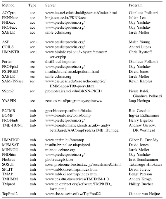
^aAcronyms: prediction of: acc—solvent accessibility; sec—secondary structure; tmb—transmembrane beta strands; tmh—transmembrane helices.

PRACTICAL ASPECTS

Evaluation of Prediction Methods Correctly Evaluating Protein Structure Prediction is Difficult

Developers of prediction methods in bioinformatics may significantly overestimate their performance because of the following reasons. First, it is difficult and time consuming to correctly separate data sets used for developing and testing. Second, estimates of performance of the different methods are often based on different data sets. This problem frequently originates from the rapid growth of the sequence and structure databases. Third, single scores are usually not sufficient to describe the performance of a method. The lack of clarity is particularly unfortunate at a time when an increasing number of tools are made easily available through the Internet and many of the users are not experts in the field of protein structure prediction. Two prominent examples illustrate this problem. (1) Trans-membrane helix predictions have been estimated to yield levels above 95% per-residue accuracy that is more than 18 percentage points above actual performance on subsequent test cases (Chen and Rost, 2002). It is not unlikely that the recent methods for the prediction of beta-barrel membrane proteins are also overestimated. (2) Many publications on predicting the secondary structural class from amino acid composition allowed correlations between “training” and testing sets. Consequently, levels of prediction accuracy published, close to 100%, exceeded by far the theoretical possible margins—around 60% (Wang and Yuan, 2000).

Although overestimates of performance can slow down experimental and theoretical progress substantially, sometimes methods perform more than anticipated by the authors. For instance, PROFtmb was published as a method that fails to identify TMB proteins in eukaryotes when used with default thresholds. Nevertheless, experimental groups have used this tool to identify eukaryotic TMB proteins. Similarly, PHDsec, PSIPRED, and PROFsec were published with the warning that they work exclusively for globular, nonmembrane proteins. There is evidence that these tools actually also work for integral membrane proteins (Forrest, Tang, and Honig, 2006).

CASP: How Well do Experts Predict Protein Structure?. Altogether seven CASP experiments have attempted to address the problem of overestimated performance (Moult et al., 1995,1997,and 1999;Zemla, Venclovas, and Fidelis, 2001; Moult et al., 2003; Moult et al., 2005). The procedure used by CASP is the following: (1) Experimentalists who are about to determine the structure of a protein send the sequence to the CASP organizers (Zemla, Venclovas, and Fidelis, 2001). (2) Sequences are distributed to the predictors. The deadline for returning results is given by the date that the structure will be published. (3) All predictions are evaluated in a meeting at Asilomar. CASP resolves the bias resulting from using known protein structures as targets. However, it often cannot provide statistically significant evaluations since the number of proteins tested is too small (Rost and Eyrich, 2001; Eyrich et al., 2001; Marti-Renom et al., 2002). Nevertheless, CASP provides valuable insights into the performance of prediction methods and has become the major source of development in the field of protein structure prediction. Due to the fact that “failing at CASP is bad for the CV,” most predictions are submitted only after experts have studied the data in detail. Thus, CASP intrinsically evaluates how well the best experts in the field can predict structure.

EVA and LiveBench: Automatic, Large-Scale Evaluation of Performance. The limitations of CASP prompted two efforts at creating large-scale and continuously running tools that automatically assess protein structure prediction servers: EVA (Eyrich et al., 2001,2003; Koh et al., 2003; Grana et al., 2005) and LiveBench (Rychlewski, Fischer, and Elofsson, 2003; Rychlewski and Fischer, 2005). LiveBench specializes in the evaluation of fold recognition, while EVA analyzes comparative modeling, contact prediction, fold recognition, and secondary structure prediction. The EVA results for secondary structure prediction methods were essential to conclude that these methods have improved significantly and to isolate the particular reasons for the improvements (mostly due to growing databases) (Rost, 2001; Rost and Eyrich, 2001; Przybylski and Rost, 2002).

Secondary Structure Prediction in Practice

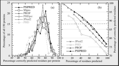
77% Right Means 33% Wrong!. The best current methods (Porter, SABLE, SAM-T04, PSIPRED, PROFphd, SSpro) reach levels around 77-80% accuracy (percentage of residues predicted correctly in one of the three states: helix, strand, or other) (Rost, 2001; Rost and Baldi, 2001; Eyrich et al., 2003; Rost, 2005). Five observations are important for using prediction methods. (1) Levels of accuracy are averages over many proteins (Figure 29.4a). Hence, the accuracy for the prediction of your protein may be much lower, or much higher, than 77%. (2) Stronger predictions are usually more accurate (Figure 29.4b). This allows, to some extent, to find out whether or not the prediction for your protein is more likely to be above or below average. (3) Often predictions go badly wrong, that is, helices are incorrectly predicted as strands and vice versa. In fact, the best current methods confuse helices and strands for, on average, about 3% of all residues (Eyrich et al., 2003). Encouragingly, some of these “bad errors” are in fact not so severe, after all, since some of these are due to regions that can switch structural conformations in response to environmental changes (see below). (4) Prediction accuracy is rather sensitive to the information contained in the alignment used for the prediction: differences between single-sequence-based predictions and optimal alignment-based predictions can exceed more than 25 percentage points (Przybylski and Rost, 2002). (5) Ifon average 77% of the residues are correctly predicted, this trivially implies that 33% are wrong. Often, it is extremely instructive to form an expert opinion about where these wrong predictions are (Hubbard et al., 1996).

Figure 29.4. Prediction accuracy varies but stronger predictions are better! All results are based on 150 novel protein structures not used to develop any of the methodshown (Eyrich et al., 2001, 2003). For all methods shown, the three-state per-residue accuracy varies significantly between these proteins, with one standard deviation in the order of 10%(a). This implies that it is difficult for users to estimate the “actual” accuracy for their protein. However, most methods now provide an index measuring the reliability of the prediction for each residue. Shown is the accuracy versus the cumulative percentages of residues predicted at a given level of reliability (coverage versus accuracy). For example, PSIPRED and PROFphd reach a level above 88% for about 60% of all residues (dashed line). This particular line is chosen since secondary structure assignments by DSSP agree to about 88% for proteins of similar structure. Although JPred2 is only marginally less accurate than PSIPRED and PROFphd, it reaches this level of accuracy for less than half of all residues.

Latest Improvement: 4 Parts Database Growth, 3 Better Search, 4 Other. Jones solicited two causes for the improved accuracy of PSIPRED: (1) training and (2) testing the method on PSI-BLAST profiles. Cuff and Barton (2000) examined in detail how different alignment methods improve. However, which fraction of the improvement results from the mere growth of the database, which from using more diverged profiles, and which from training on larger profiles? Using the PHD version from 1994 to separate the effects (Przybylski and Rost, 2002), we first compared a noniterative standard BLAST (Altschul and Gish, 1996) search against SWISS-PROT (Bairoch and Apweiler, 2000) with one against SWISS-PROT + TrEMBL (Bairoch and Apweiler, 2000) + PDB (Berman et al., 2002). The larger database improves performance by about two percentage points (Przybylski and Rost, 2002). Secondly, we compared the standard BLAST against the big database with an iterative PSI-BLAST search. This yielded less than two percentage points additional improvement (Przybylski and Rost, 2002). Thus, overall, the more divergent profile search against today’s databases supposedly improves any method using alignment information by almost four percentage points. The improvement through using PSI-BLAST profiles to develop the method is relatively small: PHDpsi was trained on a small database of not very divergent profiles in 1994; for example, PROFphd was trained on PSI-BLAST profiles of a 20 times larger database in 2000. The two differ by only one percentage point, and part of this difference resulted from implementing new concepts into PROF (Rost, 2005).

Averaging Over Many Methods May Help. All methods predict some proteins at lower levels of accuracy than others (Rost et al., 1993; Lesk et al., 2001; Rost and Eyrich, 2001). Nevertheless, for most proteins there is a method that predicts secondary structure at a level higher than average (Rost and Eyrich, 2001). The latter is applied when averaging over prediction methods. In fact, such averages are helpful as long as compiled over good methods (Rost et al., 2001). Thus, using ALL available programs is a rather bad idea!

Solvent Accessibility Prediction in Practice

Very few of the seemingly more accurate methods predicting solvent accessibility are publicly available. Furthermore, there is no EVA-like evaluation of methods based on large sets and identical conditions. The first case scenario in which methods are compared based on different data sets, and different ways to define accessibility, is the rule rather than the exception. Thus, it is important to view values published with caution. Most methods predict accessibility in two states (exposed and buried). Levels of prediction accuracy vary significantly according to choice of the thresholds to distinguish between the two states (Cuff and Barton, 2000). If we define all residues that are less than 16% solvent accessible as “exposed,” the best current methods reach levels around 75 ± 10% accuracy (Rost and Sander, 1994a; Lesk, 1997; Cuff and Barton, 2000; Przybylski and Rost, 2002). Using alignment information significantly improves prediction accuracy. However, accessibility predictions are more sensitive to alignment errors than secondary structure predictions (Rost and Sander, 1994a; Przybylski and Rost, 2002). A reason for this may be that accessibility is evolutionarily less well conserved than is secondary structure (Przybylski and Rost, 2002).

Transmembrane Region Prediction in Practice

Caution: No Appropriate Estimate of Performance Available!. The appropriate evaluation of methods predicting membrane helices is even more difficult than the evaluation of other categories of structure prediction. Three major problems prevent adequate analyses. (1) We do not have enough high-resolution structures to allow a statistically significant analysis (Chen and Rost, 2002). (2) Low-resolution experiments (gene fusion) differ from high-resolution experiments (crystallography) almost as much as prediction methods do (Chen and Rost, 2002). Thus, low-resolution experiments do not suffice to evaluate prediction accuracy. (3) All methods optimize some parameters. Since there are so few high-resolution structures, all methods use as many of the known ones, as possible. However, those methods perform much better on proteins for which they were developed than on new proteins was impressively demonstrated—and overlooked in a recent analysis of prediction methods (Moller, Croning, and Apweiler, 2001).

Crude Estimates for Where We Are at in the Field. The best current methods (HMMTOP2, PHDhtm, and TMHMM2) predict all helices correct for about 70% of all proteins (Chen and Rost, 2002). MINNOU (Cao et al., 2006) and Phobius (Kall, Krogh, and Sonnhammer, 2004, 2005) are likely to reach similar or even higher performance. For more than 60% of the proteins, the topology is also predicted correctly (Moller, Croning, and Apweiler, 2001; Chen and Rost, 2002). PHDhtm getting about 70% ofthe observed TMH residues right (Chen and Rost, 2002) achieves the most accurate per-residue prediction. All methods based on advanced algorithms tend to underestimate transmembrane helices; thus, about 86% of the TMH residues predicted by the best methods in this category PHD and DAS are correct (Chen and Rost, 2002). Most methods tend to confuse signal peptides with membrane helices; the best separation is achieved by a system predicting subcellular localization ALOM2 (Nakai and Kanehisa, 1992). Almost as accurate are PHD and TopPred2 (followed by TMHMM) (Moller, Croning, and Apweiler, 2001). Surprisingly, most methods have also been overestimated in their ability to distinguish between globular and helical membrane proteins; particularly, most methods based only on hydrophobicity scales incorrectly predict membrane helices in over 90% of a representative set of globular proteins (Chen, Kernytsky, and Rost, 2002). TMHMM, SOSUI, and PHDhtm appear to yield the most accurate distinction between membrane and globular proteins (less than 2% false positives) (Chen and Rost, 2002). The most accurate hydrophobicity index appears to be the one recently developed in the Ben-Tal group (Kessel and Ben-Tal, 2002). All methods fail to distinguish membrane helices from signal peptides to the extent that the best methods still falsely predict membrane helices for 25% (PHDhtm) to 34% (TMHMM2) of all signal peptides tested. The good news for the practical application are that we have an accurate method detecting signal peptides (Nielsen et al., 1997) and that most incorrectly predicted membrane helices start closer than 10 residues to N-terminal methionine residues, that is, could be corrected by experts.

Genome Analysis: Many Proteins Contain Membrane Helices. Despite the overestimated performance, predictions of transmembrane helices are valuable tools to quickly scan entire genomes for membrane proteins. A few groups base their results only on hydrophobicity scales, known to have extremely high error rates in distinguishing globular and membrane proteins. Nevertheless, the averages published for entire genomes are surprisingly similar between different authors (Goffeau et al., 1993; Rost, Casadio, and Fariselli, 1996; Arkin, Briinger, and Engelman, 1997; Frishman and Mewes, 1997; Jones, 1998; Wallin and vonHeijne, 1998; Liu and Rost, 2001). About 10-30% of all proteins appear to contain membrane helices. One crucial difference, however, is that more cautious estimates do not perceive a statistically significant difference in the percentage of TMH proteins across the three kingdoms: eukaryotes, prokaryotes, and archaea (Liu, Tan, and Rost, 2002). However, preferences between particular types of membrane proteins differ; in particular, eukaryotes have more 7TM proteins (receptors), whereas prokaryotes have more 6- and 12TM proteins (ABC transporters) (Wallin and von Heijne, 1998; Liu and Rost, 2001).

EMERGING AND FUTURE DEVELOPMENTS

Regions Likely to Undergo Structural Change Predicted Successfully

Young et al. (1999) have unraveled an impressive correlation between local secondary structure predictions and global conditions. The authors monitor regions for which secondary structure prediction methods give equally strong preferences for two different states. Such regions are processed combining simple statistics and expert rules. The final method is tested on 16 proteins known to undergo structural rearrangements and on a number of other proteins. The authors report no false positives, and they identify most known structural switches. Subsequently, the group applied the method to the myosin family identifying putative switching regions that were not known before but appeared reasonable candidates (Kirshenbaum, Young, and Highsmith, 1999). I find this method most remarkable in two ways: (1) it is the most general method using predictions of protein structure to predict some aspects of function and (2) it illustrates that predictions may be useful even when structures are known (as in the case of the myosin family). Recently, several group have begun to predict local flexibility directly;for example, Wiggle (Gu, Gribskov, and Bourne, 2006) identifies flexible regions through a rather unique, innovative combination of molecular dynamics and machine learning. PROFbval (Schlessinger, Yachdav, and Rost, 2006) predicts normalized B-values directly from sequence alignments through neural networks; like many recent state-of-the-art methods, PROFbval uses other 1D predictions as input. GlobPlot (Linding et al., 2003a) uses the correlation between low-complexity and flexibility.

Aspects of Protein Function Predicted by Expert Analysis of Secondary Structure

The typical scenario in which secondary structure predictions help us to learn more about function comes from experts combining predictions and their intuition, most often to find similarities to proteins of known function but insignificant sequence similarity (Brautigam et al., 1999; Davies et al., 1999; de Fays et al., 1999; DiStasio et al., 1999; Gerloff et al., 1999; Juan et al., 1999; Laval et al., 1999; Seto et al., 1999; Xu et al., 1999; Jackson and Russell, 2000; Paquet et al., 2000; Shah et al., 2000; Stawiski et al., 2000). Usually, such applications are based on very specific details about predicted secondary structure (some examples in Table 29.1). Thus, successful correlations of secondary structure and function appear difficult to incorporate into automatic methods.

Exploring Secondary Structure Predictions to Improve Database Searches

Initially, three groups independently applied secondary structure predictions to fold recognition, that is, the detection of structural similarities between proteins of unrelated sequences (Rost, 1995; Fischer and Eisenberg, 1996; Russell, Copley, and Barton, 1996). A few years later, almost every other fold recognition/threading method has adopted this concept (Ayers et al., 1999; de la Cruz and Thornton, 1999; Di Francesco, Munson, and Garnier, 1999; Hargbo and Elofsson, 1999; Jones, 1999a; Jones et al., 1999; Koretke et al., 1999; Ota et al., 1999; Panchenko, Marchler-Bauer, Bryant, 1999;Kelley,MacCallum, and Sternberg, 2000). Two recent methods extended the concept by not only refining the database search but also by actually refining the quality of the alignment through an iterative procedure (Heringa, 1999; Jennings, Edge, and Sternberg, 2001; Simossis and Heringa, 2005; Simossis, Kleinjung, and Heringa, 2005; Sammeth and Heringa, 2006). A related strategy has been explored by Ng and Henikoffs to improve predictions and alignments for membrane proteins (Ng, Henikoff, and Henikoff, 2000); the concept has been adopted by others (Muller et al., 2001; Hedman et al., 2002; Sutormin, Rakhmaninova, and Gelfand, 2003; Yu and Altschul, 2005; Sadovskaya, Sutormin, and Gelfand, 2006).

From 1D Predictions to 2D, and 3D Structure

Are secondary structure predictions accurate enough to help predict higher order aspects of protein structure automatically? 2D (inter-residue contacts) predictions: Baldi et al. (2000) have recently improved the level of accuracy in predicting beta-strand pairings over earlier work (Hubbard and Park, 1995) by using another elaborate neural network system. 3D predictions: the following list of five groups exemplifies that secondary structure predictions have now become a popular first step toward predicting 3D structure. (1) Ortiz et al. (1999) successfully use secondary structure predictions as one component of their 3D structure prediction method. (2) Eyrich and coworkers (Eyrich et al., 1999a; Eyrich, Standley, Friesner, 1999) minimize the energy of arranging predicted rigid secondary structure segments. (3) Lomize et al. (1999) also start from secondary structure segments. (4) Chen, Singh, and Altman, 1999 suggest using secondary structure predictions to reduce the complexity of molecular dynamics simulations. (5) Levitt and coworkers (Samudrala et al., 1999, 2000) combine secondary structure-based simplified presentations with a particular lattice simulation attempting to enumerate all possible folds.

Using Accessibility to Predict Aspects of Function

Features of multiple alignments can reveal aspects of protein function (Casari, Sander, and Valencia, 1995; Lichtarge, Bourne, and Cohen, 1996; Lichtarge, Yamamoto, and Cohen 1997; Pazos et al. 1997; Marcotte et al. 1999; Irving et al., 2000; Wodak and Mendez, 2004). To simplify the story, residues can be conserved because of structural and functional reasons. If we could distinguish between the two, we could predict the functional residues. Obviously, residues that are exposed and conserved are likely to reveal functional constraints. This suggests using predicted accessibility and combination with alignments to predict functional residues. One particular application is the identification of residues involved in transient protein-protein interactions (Yao et al. 2003; Wodak and Mendez 2004; Ofran and Rost 2007a; Porollo and Meller 2007). Once again, methods combining evolutionary information and 1D predictions as input perform best (Ofran and Rost 2007a); in fact, they are accurate enough to even predict interaction hot spots (Ofran and Rost 2007b). Another possible application of predicted accessibility is the prediction of subcellular localization: the surface compositions differ significantly between extracellular, cytoplasm, and nuclear proteins (Andrade, O’Donoghue, and Rost, 1998). Many methods have recently used this correlation to better the prediction of localization (Nair and Rost, 2003a; Nair and Rost, 2003b; Nair and Rost, 2004; Yu et al., 2004; Nair and Rost, 2005; Lee et al., 2006; Pierleoni et al. 2006; Rossi, Marti-Renom, and Sali, 2006). The combination of 1D predictions and predictions of localization can be used to annotate experimental protein-protein interactions as, for example, exemplified in the PiNAT system (Ofran et al., 2006) that annotates protein networks.

Using 1D Predictions for Target Selection in Structural Genomics

Structural genomics proposes to experimentally determine one high-resolution structure for every known protein (Gaasterland, 1998; Rost, 1998; Sali, 1998; Burley et al., 1999; Shapiro and Harris, 2000; Thornton, 2001). Obviously, this goal could be reached faster if we could avoid all proteins of known structure. This is relatively straightforward (Sali, 1998; Liu and Rost, 2002; Liu, Tan, and Rost, 2002). More difficult is the task of avoiding proteins that do not express, do not purify, or are longer than 200 residues, and do not crystallize (or do not diffract well enough). One way toward this goal is to exclude all proteins with membrane helices (Liu and Rost, 2001; Liu and Rost, 2002). Can bioinformatics do more than that? A whole battery of approaches is being applied to steer the target selection and structure exploitation in the operating structural genomics centers (Yao et al., 2003; Bray et al., 2004; Chelliah et al., 2004; DeWeese-Scott and Moult, 2004; Grant, Lee, and Orengo, 2004; Jones and Thornton, 2004; Liu and Rost, 2004a; Liu and Rost, 2004b; Liu et al., 2004; Nair and Rost, 2004; Chandonia and Brenner, 2005; Gutteridge and Thornton, 2005; Kifer, Sasson, and Linial, 2005; Nimrod et al., 2005; Oldfield et al., 2005b; Pal and Eisenberg, 2005; Sasson and Linial, 2005; Bhattacharya, Tejero, and Montelione, 2006; Gu, Gribskov, and Bourne, 2006; Kouranov et al., 2006; Rossi, Marti-Renom, and Sali, 2006; Levitt, 2007; Liu, Montelione, and Rost, 2007; Marti-Renom et al., 2007). Many of these approaches are based on 1D predictions.

Eukaryotes Full of Disorder?

At the point of the first edition of this book, it had been shown that regions of low-complexity, as predicted by the program SEG (Wootton and Federhen, 1996), are the rule rather than the exception in the protein universe (Saqi, 1995; Garner et al., 1998; Romero et al., 1998; Wright and Dyson, 1999; Dunker et al., 2001; Dunker and Obradovic, 2001; Romero et al., 2001). Using predictions of secondary structure, we had found that there are many proteins that do not have low-complexity regions but nevertheless appear to have long (more than 70 residues) regions without regular secondary structure (helix/strand, dubbed NORS). Such NORS proteins appear to be significantly more abundant in eukaryotes than in all other kingdoms, reaching levels around 25% of the entire genome (Liu, Tan, and Rost, 2002). We found many of the NORS to be evolutionarily conserved, suggesting that these may in fact be proteins with induced structure rather than without structure. These findings had confirmed earlier analyses (Dunker et al., 2001) and have been confirmed by subsequent work (Ward et al., 2004).

Since the publication of the first edition of the book, the field has exploded. Over the last years, many studies have shown that often the lack of a unique, native 3D structure in physiological conditions can be crucial for function (Dyson and Wright, 2004; Fuxreiter et al., 2004; Dunker et al., 2005; Dyson and Wright, 2005; Tompa, 2005; Vucetic et al., 2005; Liu et al., 2006; Radivojac et al., 2006). Such proteins are often referred to as disordered, unfolded, natively unstructured,or intrinsically unstructured proteins. A typical example is a protein that adopts a unique 3D structure only upon binding to an interaction partner and thereby performs its biochemical function (Dyson and Wright, 2004; Fuxreiter et al., 2004; Dyson and Wright, 2005). The better our experimental and computational means of identifying such proteins, the more we realize that they come in a great variety: some adopt regular secondary structure (helix or strand) upon binding, some remain loopy; some proteins are almost entirely unstructured, others have only short unstructured regions. The more our ability to recognize short unstructured regions increases, the more we realize that the label “unstructured protein” would be rather misleading, as most “unstructured proteins” have relatively short unstructured regions. There is no single one way to define “unstructured regions.” Many methods have been developed that predict such natively unstructured or disordered regions based on a great diversity of aspects (Tompa, 2002; Jones and Ward, 2003; Linding et al., 2003a; Vucetic et al., 2003; Radivojac et al., 2004; Beltrao and Serrano, 2005; Coeytaux and Poupon, 2005; Dosztanyi et al., 2005; Lise and Jones, 2005; Oldfield et al., 2005a; Gu, Gribskov, and Bourne, 2006; Vullo et al., 2006; Schlessinger, Liu, and Rost, 2007a; Schlessinger, Punta, and Rost, 2007b). Increasingly, it becomes apparent that unstructured regions are an important means of increasing complexity of molecular interactions. It is rather remarkable that methods developed for the prediction of regular 1D structure become once again crucial for the exploration of regions that appear to pose an altogether different challenge to the advance of structural biology over the next decade.