30
HOMOLOGY MODELING
INTRODUCTION
The goal of protein modeling is to predict a structure from its sequence with an accuracy that is comparable to the best results achieved experimentally. This would allow users to safely use in silico generated protein models in scientific fields where today only experimental structures provide a solid basis: structure-based drug design, analysis of protein function, interactions, antigenic behavior, or rational design of proteins with increased stability or novel functions. Protein modeling is the only way to obtain structural information when experimental techniques fail. Many proteins are simply too large for NMR analysis and cannot be crystallized for X-ray diffraction.
Among the three major approaches to 3D structure prediction described in this and the following two chapters, homology modeling is the “easiest” approach based on two major observations:
- The structure of a protein is uniquely determined by its amino acid sequence (Epstain, Goldberger, and Anfinsen, 1963), and therefore the sequence should, in theory, contain suffice information to obtain the structure.
- During evolution, structural changes are observed to be modified at a much slower rate than sequences. Similar sequences have been found to adopt practically identical structures while distantly related sequences can still fold into similar structures. This relationship was first identified by Chothia and Lesk (1986) and later quantified by Sander and Schneider (1991), as summarized in Figure 30.1. Since the initial establishment of this relationship, Rost et al. were able to derive a more precise limit for this rule with accumulated data in the PDB (Rost, 1999). Two protein sequences are highly likely to adopt a similar structure provided that the percentage identity between these proteins for a given length is above the threshold shown in Figure 30.1.
Figure 30.1. The two zones of sequence alignments defining the likelihood of adopting similar structures. Two sequences are highly likely to fold into the same structure if their length and percentage sequence identity fall into the region above the threshold, indicated with the smiling icon (the “safe” zone). The region below the threshold indicates the zone where inference of structural similarity cannot be made, thus making it difficult to determine if model building will be possible. Figure based on Sander and Schneider (1991).
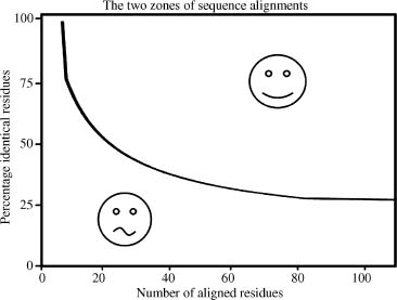
The identity between the sequences can be obtained by doing a simple BLAST run with the sequence of interest, the model sequence, against the PDB, see Figure 30.2. The sequence that aligns with the model sequence is called the “template.” When the percentage identity in the aligned region of the structure template and the sequences to be modeled falls in the safe modeling zone of Figure 30.1, a model can be built. It is shown in Figure 30.1 that the threshold for safe homology modeling can be as low as 25%, especially for longer sequences. However, the quality of the model is dependent on the sequence identity and should be considered since sequences with 25% sequence identity tend to yield poor structural models with high uncertainty in side chain positioning.
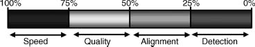
The impact of identities between the model sequence and the template on the process of protein homology modeling can be broken down as follows. At sequence identities greater than 75%, protein homology modeling can easily be achieved requiring minor manual intervention. Consequently, the time needed to finalize such a model is limited only by the interpretation of the model to answer the biological question at hand, see Figure 30.3. The level of accuracy achieved with these models is comparable to structures that were solved by NMR. For sequence identities between 50% and 75%, more time is needed to fine-tune the details of the model and correct the alignment if needed. Between 25% and 50% identity obtaining the best possible alignment becomes the concern in the process of homology modeling. Finally, sequence identities lower than 25% often mean that no template structure can be detected with a simple BLAST search, thus requiring the use of more sensitive alignment techniques (Chapter 31), to find a potential template structure.
Figure 30.2. Typical blast output of a model sequence run against the PDB sequences, where Q represents the model sequence with unknown structure and S is the sequence for the PDB structure template.
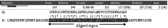
Figure 30.3. The limiting steps in homologymodeling as function of percentage sequence identity between the model sequence and the sequence of the template. Figure based on Rodriguez and Vriend (1997).
In practice, homology modeling is a multistep process that can be summarized as follows:
1.Template recognition and initial alignment
2.Alignment correction
3.Backbone generation
4.Loop modeling
5.Side chain modeling
6.Model optimization
7.Model validation
8.Iteration
These steps are all illustrated in Figure 30.4 and will be discussed in detail in the rest of this chapter.
Decisions need to be made by the modeler at almost every step of this model building process. The choices are not always obvious, thus subjecting model building to a serious thought about how to gamble between multiple seemingly similar choices. To reduce possible errors introduced by a subjective decision making process, algorithms have been developed to automate the model building process (Table 30.1).
Current techniques allow modelers to construct models for about 25-65% of the amino acids coded in the genome, thereby supplementing the efforts of structural genomics projects (Xiang, 2006). This value differs significantly between individual genomes and increases steadily with the continuous growth of the PDB. The remaining 75-35% of these genomes have no identified template that can be used for homology modeling and therefore modelers will need to resort to fold recognition (Chapter 31), ab initio structure prediction (Chapter 32), or simply the traditional NMR or X-ray experiment to obtain structural data (Chapters 4 and 5). While automated model building provides a high-throughput solution, the evaluation of these automated methods during CASP (Chapter 28) indicated that human expertise is still helpful, especially if the sequence identity of the alignment is close to the zone of uncertainty regarding the feasibility of building a proper model (25%, see Figure 30.1) (Fischer et al., 1999). The eight steps of homology modeling will be discussed below in more detail.
Figure 30.4. The process of building a “model” by homology to a “template.” The numbers in the plot correspond to the step numbers in the subsequent section. (Colored version of this Figure is available for viewing at http://swift.cmbi.ru.nl/material/)
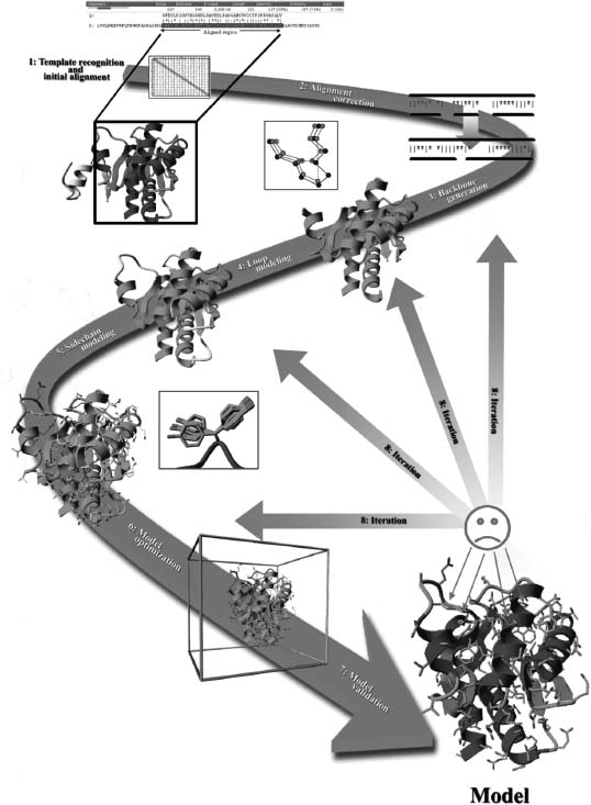
TABLE 30.1 A Few Examples of the Online Available Homology Modeling Servers
| Server Name | URL | |
| Automatic Homology Modeling Servers | ||
| 3D-Jigsaw | http://www.bmm.icnet.uk/servers/3djigsaw/ | |
| CPHModels | http://www.cbs.dtu.dk/services/CPHmodels/ | |
| EsyPred3D | http://www.fundp.ac.be/urbm/bioinfo/esypred/ | |
| Robetta | http://robetta.bakerlab.org/ | |
| SwissModel | http://swissmodel.expasy.org/ | |
| TASSER-lite | http://cssb.biology.gatech.edu/skolnick/webservice/tasserlite/index.html | |
| Semiautomatically Homology Modeling Servers | ||
| HOMER | http://protein.cribi.unipd.it/homer/help.html | |
| WHAT If | http://swift.cmbi.kun.nl/WIWWWI/ | |
STEP 1—TEMPLATE RECOGNITION AND INITIAL ALIGNMENT
Sequences in the safe homology modeling zone (Figure 30.1) share high percentage identity to a possible template and therefore can easily be paired with simple sequence alignment programs such as BLAST (Altschul et al., 1990) or FASTA (Pearson, 1990).
To identify the template, the program compares the query sequence to all the sequences of known structures in the PDB mainly using two matrices:
- A Residue Exchange Matrix (Figure 30.5). This matrix defines the likelihood that any 2 of the 20 amino acids ought to be aligned. Exchanges between different residues with similar physicochemical properties (e.g., F ! Y) get a better score than exchanges between residues that widely differ in their properties. Conserved residues generally obtain the highest score.
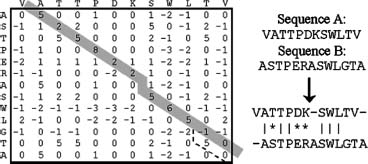
- An Alignment Matrix (Figure 30.6). The axes of this matrix correspond to the two sequences to be aligned, and the matrix elements are simply the values from the residue exchange matrix (Figure 30.5) for a given pair of residues. During the alignment process, one tries to find the best path through this matrix, starting from a point near the top left and going down to the bottom right. To make sure that no residue is used twice, one must always take at least one step to the right and one step down. A typical alignment path is shown in Figure 30.6. At first sight, the dashed path in the bottom right corner would have led to a higher score. However, it requires the opening of an additional gap in sequence A (Gly of sequence B is skipped). By comparing thousands of sequences and sequence families, it became clear that the opening of gaps is about as unlikely as at least a couple of nonidentical residues in a row. The jump roughly in the middle of the matrix on the other hand is justified, because after the jump we earn lots of points (5, 6, 5) that otherwise would only have been (1,0, 0). The alignment algorithm therefore subtracts an ’’opening penalty’’ for every new gap and a much smaller ’’gap extension penalty’’ for every residue that is additionally skipped once the gap has already been made. The gap extension penalty is much smaller than the gap open penalty because one gap of three residues is much more likely than three gaps of one residue each.
Figure 30.5. A typical residue exchange or scoring matrix used by alignment algorithms. Because the score for aligning residues A and B is normally the same as for B and A, this matrix is symmetric.

Figure 30.6. The alignment matrix for the sequences VATTPDKSWLTV and ASTPERASWLGTA, using the scores from Figure 30.3. The optimum path corresponding to the alignment on the right side is shown in gray. Residues with similar properties are marked with a star “*’’. The dashed line marks an alternative alignment that scores more points but requires to open a second gap.
In practice, template structures can be easily retrieved by submitting the query sequence to one of the countless BLAST servers on the web, using the PDB as the database to search. Usually, the template structure with the highest sequence identity will be the first option, see Figure 30.2, but other considerations should also be made. For example, the conformational state (i.e., active or inactive), present cofactors, other molecules, or multimeric complexes will have an impact on model building. Nowadays, the increasing amount of CPU power makes it possible to choose multiple templates and build multiple models giving the investigator the opportunity to select the best model for further study. It has also become possible to combine multiple templates into one structure that is used for modeling. The online Swiss-Model and the Robetta servers, for example, use this approach (Peitsch, Schwede, and Guex, 2000; Kim, Chivian, and Baker, 2004).
STEP 2—ALIGNMENT CORRECTION
Having identified one or more possible modeling templates using the initial screen described above, more sophisticated methods are needed to arrive at a better alignment.
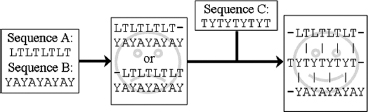
Sometimes it may be difficult to align two sequences in a region where the percentage sequence identity is very low. A potential strategy is to use other sequences from other homologous proteins to find a solution. An example of using this strategy to address a challenging alignment is shown in Figure 30.7. Suppose the sequence LTLTLTLT needs to be aligned with YAYAYAYAY. There are two equally poor possibilities, and the use of third sequence, TYTYTYTYT, that aligns to the two sequences can resolve the issue.
Figure 30.7. Addressing a challenging alignment problem with homologous sequences. Sequences A and B are impossible to align, unless one considers a third sequence C from a homologous protein.
The example mentioned above introduced a very powerful concept called ’’multiple sequence alignment.’’ Many programs are available to align a number of related sequences, for example, ClustalW (Thompson, Higgins, and Gibson, 1994), and the resulting alignment contains a lot of additional information. Think about an Ala → Glu mutation. Relying on the matrix in Figure 30.5, this exchange always gets a score of 1. In the three-dimensional structure of the protein, it is however very unlikely to see such an Ala → Glu exchange in the hydrophobic core, but on the surface this mutation is perfectly normal. The multiple sequence alignment implicitly contains information about this structural context. If at a certain position only exchanges between hydrophobic residues are observed, it is highly likely that this residue is buried. To consider this knowledge during the alignment, one uses the multiple sequence alignment to derive position specific scoring matrices, also called ’’profiles’’ (Taylor, 1986; Dodge, Schneider, and Sander, 1998). During the past years, new programs such as MUSCLE and T-Coffee have been developed that use these profiles to generate and refine the multiple sequence alignments. (Notredame, Higgins, and Heringa, 2000; Edgar, 2004). Structure-based alignments programs, such as 3DM, also include structural information in combination with profiles to generate multiple sequence alignments (Folkertsma et al., 2004). The use of 3DM on a specific class of proteins can result in entropy versus variability plots. The location of a residue in this plot is directly related to function in the protein. This information can in turn be added to the profile and used to correct the alignment or to optimize position specific gap penalties.
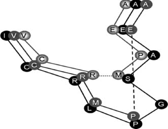
When building a homology model, we are in the fortunate situation of having an almost perfect profile—the known structure of the template. We simply know that a certain alanine sits in the protein core and must therefore not be aligned with a glutamate. Multiple sequence alignments are nevertheless useful in homology modeling, for example, to place deletions or insertions only in areas where the sequences are strongly divergent. A typical example for correcting an alignment with the help of the template is shown in Figures 30.8 and 30.9. Although a sequence alignment gives the highest score for alignment 1 in Figure 30.8, a simple look at the structure of the template reveals that alignment 2 is actually a better alignment, because it leads to a small gap compared to a huge hole associated with alignment 1.
Figure 30.8. Example of a sequence alignment where a three-residue deletion must be modeled. While alignment 1, dark gray, appears better when considering just the sequences (a matching proline at position 5), a look at the structure of the template leads to a different conclusion (Figure 30.9).
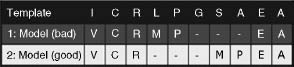
Figure 30.9. Correcting an alignment based on the structure of the modeling template (Cα trace shown in black). While the alignment with the highest score (dark gray, also in Figure 30.8) leads to a big gap in the structure, the second option (light gray) creates only a tiny hole. This can easily be accommodated by small backbone shifts.
STEP 3—BACKBONE GENERATION
When the alignment is ready, the actual model building can start. Creating the backbone is trivial for most of the models: one simply transfers the coordinates of those template residues that show up in the alignment with the model sequence (see Figure 30.2). If two aligned residues differ, the backbone coordinates for N, Cα,C,and O, and often also Cβ can be copied. Conserved residues can be copied completely to provide an initial guess.
Experimentally determined protein structures are not perfect (but still better than models in most cases). There are countless sources of errors, ranging from poor electron density in the X-ray diffraction map to simple human errors when preparing the PDB file for submission. A lot of work has been spent on writing software to detect these errors (correcting them is even harder), and the current count is at more than 25,000,000 errors in the approximately 50,000 structures deposited in the PDB by the end of 2007. The current PDB-redo and RECOORD projects have, respectively, shown that re-refinement of X-ray and NMR structures normally improves the quality of the structure, suggesting that re-refinement before modeling seems to be a wise option (Nederveen, 2005; Joosten, 2007).
A straightforward way to build a good model is to choose the template with the fewest errors (the PDBREPORT database (Hooft et al., 1996) at www.cmbi.ru.nl/gv/pdbreport can be very helpful). But what if two templates are available, and each has a poorly determined region, but these regions are not the same? One should clearly combine the good parts of both templates in one model—an approach known as multiple template modeling. (The same applies if the alignments between the model sequence and possible templates show good matches in different regions.) Although this is simple in principle (and used by automated modeling servers like Swiss-Model (Peitsch et al., 2000)), it is hard in practice to achieve results that are closer to the true structure than all the templates. Nevertheless, the feasibility of this strategy has already been demonstrated by Andrej Šali’s group in CASP4 (Chapter 28).
One extreme example of a program that combines multiple templates is the Robetta server. This server uses several different algorithms to predict domains in the sequence. The regions of the model sequence that contain a homologous domain in the PDB are modeled while those parts without are predicted de novo by using the Rosetta method. This method compares small fragments of the sequence with the PDB and inserts them with the same local conformation into the model. The Robetta server can generate models of complete sequences even without a known template (Kim et al., 2004). Skolnick’s TASSER follows a same strategy but combines larger fragments, found by threading, and folds them into a complete structure (Zhang and Skolnick, 2004).
STEP 4—LOOP MODELING
For the majority of homology model building cases, the alignment between model and template sequence contains gaps, either in the model sequence (deletions as shown in Figures 30.8 and 30.9) or in the template sequence (insertions). Gaps in the model sequence are addressed by simply omitting residues from the template, thus creating a hole in the model that must be closed. Gaps in the template sequences are treated by inserting the missing residues into the continuous backbone. Both cases imply a conformational change of the backbone. The good news is that conformational changes often do not occur within regular secondary structure elements. Therefore, it is often safe to shift all insertions or deletions in the alignment out of helices and strands and place them in structural elements that can accommodate such changes in the alignment such as loops and turns. The bad news is that changes in loop conformation are notoriously hard to predict (a big unsolved problem in homology modeling). To make things worse, even without insertions or deletions a number of different loop conformations can be observed between the template and the model. Three main reasons for this difficulty can be attributed to the following reasons (Rodriguez and Vriend, 1997):
- Surface loops tend to be involved in crystal contacts and therefore a significant conformational change is expected between the template in crystal form and the final structure modeled in the absence of crystallization constraints.
- The exchange of small to bulky side chains underneath the loop induces a structural change by pushing it away from the protein.
- The mutation of a loop residue to proline or from glycine to any other residue will result in a decrease in conformational flexibility. In both cases, the new residue must fit into a more restricted area in the Ramachandran plot, which normally requires a conformational change of the loop.
There are three main approaches to model loops:
- Knowledge Based: A search is made through the PDB for known loops containing end points that match the residues between which the loop is to be inserted. The identified coordinates of the loop are then transferred. All major molecular modeling programs and servers support this approach (e.g., 3D-Jigsaw (Bates and Sternberg, 1999), Insight (Dayringer, Tramontano, and Fletterick, 1986), Modeller (Sali and Blun-dell, 1993), Swiss-Model (Peitsch et al., 2000), or WHAT IF (Vriend, 1990)).
- In Between or Hybrid: The loop is divided in small fragments that are all separately compared to the PDB. This strategy has been described earlier as implemented for the Rosetta method (Kim et al., 2004). The local conformation of all small fragments results in an ab initio modeled loop but is still based on known protein structures. This method is reminiscent of the very old ECEPP software by the Scheraga group (Zimmerman et al., 1977).
- Energy Based: As in true ab initio fold prediction, an energy function is used to judge the quality of a loop. This is followed by a minimalization of the structure, using Monte Carlo (Simons et al., 1999) or molecular dynamics techniques (Fiser, Do, and Sali, 2000) to arrive at the best loop conformation. Often the energy function is modified (e.g., smoothed) to facilitate the search (Tappura, 2001).
For short loops (up to 5-8 residues), the various methods have a reasonable chance of predicting a loop conformation close to the true structure. As mentioned above, surface loops tend to change their conformation due to crystal contacts. So if the prediction is made for an isolated protein and then found to differ from the crystal structure, it might still be correct.
STEP 5—SIDE CHAIN MODELING
When we compare the side chain conformations (rotamers) of residues that are conserved in structurally similar proteins, we find that they often have similar χ1-angles (i.e., the torsion angle about the Cα-Cβ bond). It has been shown by Summers et al. that in homologous proteins (over 40% identity) at least 75% of the Cy occupy the same orientation (Summers, Carlson, and Karplus, 1987). It is therefore possible to simply copy conserved residues entirely from the template to the model (see also Step 3) and achieve a very good starting point for structure optimization. In practice, this rule of thumb holds only at high levels of sequence identity, when the conserved residues form networks of contacts. When they get isolated (<35% sequence identity), the rotamers of conserved residues may differ in up to 45% ofthe cases (Sanchez and Sali, 1997).
In practice, all successful approaches to side chain placement are at least partly knowledge based. Libraries of common rotamers extracted from high-resolution X-ray structures are often used to position side chains. The various rotamers are successively explored and scored with a variety of energy functions. Intuitively, one might expect rotamer prediction to be computationally demanding due to the combinatorial explosion of the search space—the choice of a certain rotamer automatically affects the rotamers of all neighboring residues, which in turn affect their neighbors and the effect propagates continuously. For a sequence of 100 residues and an average ~5 rotamers per residue, the rotamer space would yield 5100 different possible conformations to score. Significant research efforts have been invested to develop algorithms to address this issue and make the search through the rotamer conformation space more tractable (e.g., Desmet et al., 1992; Canutescu, Shelenkov, and Dunbrack, 2003).
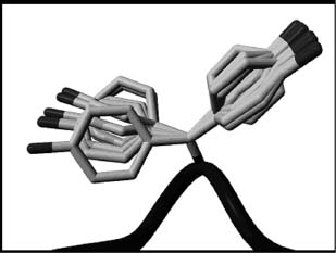
Aside from directly extracting conserved rotamers from the template, the key to handling the combinatorial explosion of conformational possibilities lies in the protein backbone. Instead of using a ’’fixed’’ library that stores all possible rotamers for all residue types, an alternative ’’position specific’’ library can be used. These libraries utilize information contained in the backbone to select the correct rotamer. A simple form of a position-specific library classifies the backbone based on secondary structure since residues found in helices often favor a rotamer conformation that is not observed in strands or turns. More sophisticated position-specific libraries can be built by classifying the backbone according to its Phi/Psi angles or by analyzing high-resolution structures and collecting all stretches of 5-9 residues (depending on the method) with reference amino acid at the center of the stretch. These collected examples in the template are superposed on the corresponding backbone to be modeled. The possible side chain conformations are selected from the best backbone matches (Chinea et al., 1995). Since certain backbone conformations will be strongly favored for certain rotamers to be adopted (allowing, for example, a hydrogen bond between side chain and backbone), this strategy greatly reduces the search space. For a given backbone conformation, there may be a residue that strongly populates a specific rotamer conformation and therefore can be modeled immediately. This residue would then serve as an anchor point to model surrounding side chains that may be more flexible and adopt a number of other conformations. An example for a backbone conformation that favors two different tyrosine rotamers is shown in Figure 30.10. Position-specific rotamer libraries are widely used today for drug docking purposes to visualize all possible shapes of the active site (de Filippis, Sander, and Vriend, 1994; Dunbrack and Karplus, 1994; Stites, Meeker, and Shortle, 1994). The study by Chinea et al. shows that the search space is even considerably smaller than assumed by Desmet et al.
Figure 30.10. Example of a backbone-dependent rotamer library. The current backbone conformation favors two different rotamers for tyrosine (shown as sticks), which appear about equally often in the database.
Although search space for rotamer prediction initially presented a combinatorial problem to be explored exhaustively, it is far smaller than originally believed as evidenced in a study conducted in 2001. Xiang and Honig first removed a single side chain from known structures and repredicted it. In a second step, they removed all the side chains and added them again using the same method. Surprisingly, it turned out that the accuracy was only marginally higher in the much easier first case (Xiang and Honig, 2001).
Rotamer prediction accuracy is usually quite high for residues in the hydrophobic core where more than 90% of all χ1-angles fall within ±20° from the experimental values, but much lower for residues on the surface where the percentage is often even below 50%. There are three reasons for this:
- Experimental Reasons: Flexible side chains on the surface tend to adopt multiple conformations, which are additionally influenced by crystal contacts. So even experiments cannot provide one single correct answer.
- Theoretical Reasons: The energy functions used to score rotamers can easily handle the hydrophobic packing in the core (mainly Van der Waals interactions). The calculation of electrostatic interactions on the surface, including hydrogen bonds with water molecules and associated entropic effects, is more complicated. Nowadays, these calculations are being included in more force fields that are used to optimize the models (Vizcarra and Mayo, 2005).
- Biological Reasons: Loops on the surface often adopt different conformations as part of the biological function, for example, to let the substrate enter the protein.
It is important to note that the rotamer prediction accuracies given in most publications cannot be reached in real-life applications. This is simply due to the fact that the methods are evaluated by taking a known structure, removing the side chains, and repredicting them. The algorithms thus rely on the correct backbone, which is not available in homology modeling since the backbone of the template often differs significantly from the model structure. The rotamers must thus be predicted based on a ’’wrong’’ backbone, and reported prediction accuracies tend to be higher than what would be expected for the modeled backbone.
STEP 6—MODEL OPTIMIZATION
The problem of rotamer prediction mentioned above leads to a classical ’’chicken and egg’’ situation. To predict the side chain rotamers with high accuracy, we need the correct backbone, which in turn depends on the rotamers and their packing. The common approach to address this problem is to iteratively model the rotamers and backbone structure. First, we predict the rotamers, remodel the backbone to accommodate rotamers, followed by a round of refitting the rotamers to the new backbone. This process is repeated until the solution converges. This boils down to a series of rotamer prediction and energy minimization steps. Energy minimization procedures used for loop modeling are applied to the entire protein structure, not just an isolated loop. This requires an enormous accuracy in the energy functions used, because there are many more paths leading away from the answer (the model structure) than toward it. This is why energy minimization must be used carefully. At every minimization step, a few big errors (like bumps, i.e., too short atomic distances) are removed while at the same time many small errors are introduced. When the big errors are gone, the small ones start accumulating and the model moves away from its correct structure, see Figure 30.11.
As a rule of thumb, today’s modeling programs therefore either restrain the atom positions and/or apply only a few hundred steps of energy minimization. In short, model optimization does not work until energy functions (force fields) become more accurate. Two ways to achieve better energetic models for energy minimization are currently being pursued:
- Quantum Force Fields: Protein force fields must be fast to handle these large molecules efficiently; energies are therefore normally expressed as a function of the positions of the atomic nuclei only. The continuous increase of computer power has now finally made it possible to apply methods of quantum chemistry to entire proteins, arriving at more accurate descriptions of the charge distribution (Liu et al., 2001). It is however still difficult to overcome the inherent approximations of today’s quantum chemical calculations. Attractive Van der Waals forces are, for example, so hard to treat, that they must often be completely omitted. While providing more accurate electrostatics, the overall accuracy achieved is still about the same as in the classical force fields.
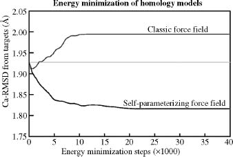
- Self-Parameterizing Force Fields: The accuracy of a force field depends to a large extent on its parameters (e.g., Van derWaals radii, atomic charges). These parameters are usually obtained from quantum chemical calculations on small molecules and fitting to experimental data, following elaborate rules (Wang, Cieplak, and Kollman, 2000). By applying the force field to proteins, one implicitly assumes that a peptide chain is just the sum of its individual small molecule building blocks—the amino acids. Alternatively, one can just state a goal—for example, improve the models during an energy minimization—and then let the force field parameterize itself while trying to optimally fulfill this goal (Krieger, Koraimann, and Vriend, 2002; Krieger et al., 2004). This leads to a computationally rather expensive procedure. Take initial parameters (e.g., from an existing force field), change a parameter randomly, energy minimize models, see if the result improved, keep the new force field if yes, otherwise go back to the previous force field. With this procedure, the force field accuracy increases enough to go in the right direction during an energy minimization (Figure 30.11), but experimental accuracy is still far out of reach.
Figure 30.11. The average RMSD between models and the real structures during an extensive energy minimization of 14 homology models with two different force fields. Both force fields improve the models during the first ~500 energy minimization steps, but then the small errors sum up in the classic force field and guide the minimization in the wrong direction, away from the real structure, while the self-parameterizing force field goes in the right direction. To reach experimental accuracy, the minimization would have to proceed all the way down to ~0.5A, which is the uncertainty in experimentally determined coordinates.
The most straightforward approach to model optimization is to simply run a molecular dynamics simulation of the model. Such a simulation follows the motions of the protein on a femtosecond (10-15 s) time scale and mimics the true folding process. One thus hopes that the model will complete its folding and converges to the true structure during the simulation. The advantage is that a molecular dynamics simulation implicitly contains entropic effects that are otherwise hard to treat; the disadvantage is that the force fields are again not accurate enough to make it work.
Different distributed computing projects, including folding@home (http://folding. stanford.edu), Rosetta@home (http://boinc.bakerlab.org/rosetta/), and Models@home (http://www.cmbi.kun.nl/models), have been developed to use many personal computers in a network to run molecular dynamics simulations and to mimic protein folding. Model optimization becomes more and more important. Even the focus of the CASP competition (Chapter 28) is changing to a comparison of the optimization of initial models provided by these online servers instead of building the initial models from scratch.
STEP 7—MODEL VALIDATION
Every protein structure contains errors, and homology models are no exception. The number of errors (for a given method) mainly depends on two values:
- The Percentage Sequence Identity Between Template and Model Sequence. If the identity is greater than 90%, the accuracy of the model can be compared to crystallo-graphically determined structures, except for a few individual side chains (Chothia and Lesk, 1986; Sippl, 1993). From 50% to 90% identity, the root mean square error in the modeled coordinates can be as large as 1.5 A, with considerably larger local errors. If the sequence identity drops to 25%, the alignment turns out to be the main bottleneck for homology modeling, often leading to very large errors rendering it a meaningless effort to model these regions, see also Figure 30.3.
- The Number of Errors in the Template. Errors in the template structure can be reduced by an additional re-refinement of the template structure as mentioned earlier. Errors in a model become less of a problem if they can be localized. For example, a loop located distantly from a functionally important region such as the active site of an enzyme can tolerate some inaccuracies. Nevertheless, it is in the best interest to model all regions as accurately as possible since seemingly unimportant residues may be important for protein-protein interactions or a yet unassigned function.
There are two principally different ways to estimate errors in a structure:
(a) Calculating the Model’s Energy Based on a Force Field. This checks if the bond lengths and bond angles are within normal ranges, and if there are lots of clashing side chains in the model (corresponding to a high Van der Waals energy). Essential questions like ’’Is the model folded correctly?’’ cannot yet be answered this way, because completely misfolded but well-minimized models often reach the same force field energy as the correct structure (Novotny, Rashin, and Bruccoleri, 1988). This is mainly due to the fact that molecular dynamics force fields are lacking several contributing terms to the energy function, most notably those related to solvation effects and entropy.
(b) Determination of Normality Indices that describe how well a given characteristic of the model resembles the same characteristic in real structures. Many features of protein structures are well suited for normality analysis. Most of them are directly or indirectly based on the analysis of interatomic distances and contacts. Some published examples are the following:
- General checks for the normality of bond lengths, bond, and torsion angles (Morris et al., 1992; Czaplewski et al., 2000) are good checks for the quality of experimentally determined structures, but are less suitable for the evaluation of models because the better model building programs simply do not make this kind of errors.
- Inside/outside distributions of polar and apolar residues can be used to detect completely misfolded models (Baumann, Frommel, and Sander, 1989).
- The radial distribution function for a given type of atom (i.e., the probability to find certain other atoms at a given distance) can be extracted from the library of known structures and converted into an energy-like quantity called a ’’potential of mean force’’ (Sippl, 1990). Such a potential can easily distinguish good contacts (e.g., between a Cγ of valine and a Cδ of isoleucine) from bad ones (e.g., between the same Cγ of valine and the positively charged amino group of lysine).
- The direction of atomic contacts can also be accounted for in addition to interatomic distances. The result is a three-dimensional distribution of functions that can also easily identify misfolded proteins and are good indicators of local model building problems (Vriend and Sander, 1993).
Most methods used for the verification of models can also be applied to experimental structures (and hence to the templates used for model building). A detailed verification is essential when trying to derive new information from the model, either to interpret or predict experimental results or to plan new experiments.
STEP 8—ITERATION
When errors in the model are recognized and located, they can be corrected by iterating portions of the homology modeling process. Small errors that are introduced during the optimization step can be removed by running a shorter molecular dynamics simulation. A error in a loop can be corrected by choosing another loop conformation in the loop modeling step. Large mistakes in the backbone conformation sometimes require the complete process to be repeated with another alignment or even with a different template.
In summary, it is safe to say that homology modeling is unfortunately not as easy as stated in the beginning. Ideally, homology modeling also uses threading (Chapter 31) to improve the alignment, ab initio folding (Chapter 32) to predict the loops, and molecular dynamics simulations with a perfect energy function to converge into the true structure. Doing all this correctly will keep researchers busy for a long time, leaving lots of fascinating discoveries.
ACKNOWLEDGMENTS
We thank Rolando Rodriguez, Chris Spronk, Sander Nabuurs, Robbie Joosten, Maarten Hekkelman, David Jones, and Rob Hooft for stimulating discussions, practical help, and critically reading the document. We apologize to the numerous crystallographers who made all this work possible by depositing structures in the PDB for not referring to each of the 50,000 very important articles describing these structures.