33

RNA STRUCTURAL BIOINFORMATICS

Magdalena A. Jonikas, Alain Laederach, and Russ B. Altman

INTRODUCTION

RNA molecules play a range of roles in cells, including key roles in both transcription and translation. Functional RNAs can have complex three-dimensional structures or simply rely on the properties of their primary sequence to perform their function. Among the highly structured RNAs are transfer RNAs (tRNA), ribosomal RNAs (rRNA), ribozymes and riboswitches. These classes of RNAs play catalytic or structural roles in the cell, facilitated by their complex three-dimensional structures. Other RNAs, such as micro-RNAs and sno-RNAs, perform their regulatory function by relying on simple base pairing to target RNAs.

Three levels of structure can exist in RNA, the primary sequence, secondary structure and tertiary structure, with each structural level serving an essential role in the function of RNA. The structure of RNA is covered extensively in Chapter 3; however, we will discuss briefly these different structural levels using tRNA to illustrate these principles. At the primary sequence level, four bases serve as the main components: adenine, guanine, cytosine, and uracil (a pyrimidine similar to the thymine found in DNA). In addition to this basic set, many modified bases such as pseudouridine and even the DNA base thymine are frequently present in RNA molecules. Figure 33.1a shows several primary sequences of molecules in the tRNA family in a multiple sequence alignment.

The secondary structure units of RNA are duplexes and loops. RNA duplexes, also called helices or stems, are formed when complementary regions within the molecule bind to form a right-handed helix. Hydrogen bonds between two complementary bases, as well as stacking interactions, stabilize the helical structure. Loops are regions of the RNA molecule that do not form a duplex. Figure 33.1b is a dot plot showing interacting residues and Figure 33.1c shows a secondary structure map for a tRNA molecule where groups of base pairs form four helices.

The tertiary structure of an RNA molecule is the interaction of duplexes and loops to form a compact three-dimensional structure. Intramolecular base pairing between nucleotides can result in structures more complex than helices. These structures include pseudoknots that occur when a loop at the end of a hairpin helix participates in another helical region. These hydrogen bonded pairing interactions are not always part of a helix and often form long-range tertiary interactions instead. Occasionally, three different nucleotides will be observed to form hydrogen bonding interactions with each other resulting in a triple pair. Figure 33.1d shows the tertiary structure of a tRNA molecule, solved by X-ray crystallography.

The history of RNA structure models begins with Michael Levitt’s remarkable 1969 prediction of the tRNA molecule’s three-dimensional structure, which was largely based on phylogenetic analysis (Levitt, 1969). Since then, a number of structured RNAs, including tRNA, have been solved by X-ray crystallography and Nuclear Magnetic Resonance (NMR) (Kim et al., 1972; Kim et al., 1973; Laederach, 2007). Today, several hundred X-ray and NMR elucidated RNA structures, mostly of small RNA fragments, can be found in both the Protein Data Bank (PDB) and the Nucleic Acid Data Bank (NDB) (Berman et al., 2002). However, because they are large and flexible, determining the structures of larger RNAs by X-ray crystallography is challenging, leaving computational modeling of RNA structure as an attractive alternative.

Prior to discussing RNA structure models, we must first address the key similarities and differences between RNA, DNA, and protein structure. Although RNA is similar to DNA in composition, one small difference in the chemistry of the sugar results in significant structural differences. The RNA backbone contains ribose, instead of the deoxyribose found in DNA, which contains one more hydroxyl group than deoxyribose, attached in the 2’ position, allowing more flexibility in the RNA backbone. This flexibility contributes to the large variety of structures that RNA can adopt whereas DNA is generally found only in double-stranded helical structures. In addition, RNA is typically a single-stranded molecule with duplex structures forming between regions within the same molecule. These duplexes can be found throughout an RNA molecule, packing together to form a three-dimensional structure. As a result, RNA molecules can adopt highly complex structures that enable them to participate in cell regulation functions.

Functional RNA molecules are similar to proteins in their ability to adopt complex three-dimensional structures in order to catalyze chemical reactions. However, there are significant differences between RNA and protein structures. Proteins are made up of 20 amino acids that vary in size, shape, polarity, and charge whereas RNA is made up of four very similar bases. This is a significant difference, because we can use our understanding of the interactions between the diverse protein building blocks, such as hydrophobic collapse, to gain insight into protein folding and structure. However, in RNA the negatively charged backbone interacts with cations in solution to form a compact structure (Heilman-Miller, et al., 2001 Heilman-Miller, Thirumalai, and Woodson, 2001; Russell et al., 2002; Williamson, 2005).

METHODS FOR PREDICTING SECONDARY STRUCTURES

As new noncoding DNA segments of the genome are discovered, scientists typically want to know the secondary structure of the corresponding RNA molecule in an attempt to elucidate their functional roles. Furthermore, there is growing evidence that most genomic sequences are transcribed resulting in a large amount of functional RNA in the cell (Eddy, 2002). Although experimental assays such as DMS footprinting are a gold standard for secondary structure determination, they are also difficult, noisy, and expensive, rendering them prohibitive for such high-throughput applications (Galas and Schmitz, 1978; Inoue and Cech, 1985; Tullius, 1988). Computational prediction offers an alternative to experimental methods and opens up the opportunity to scan new RNA sequences for secondary structures (Table 33.1).

Phylogenetic Analysis of Base Pair Covariation

Phylogenetic analysis reveals the selective pressure to maintain the base pair relationships and therefore analysis of base pair covariation can be used to define intramolecular topology. Phylogenetic analysis of RNA secondary structure uses a multiple sequence alignment of an RNA family to determine base pairs through their covariance (Fox and Woese, 1975; Woese et al., 1980; Woese et al., 1983). Figure 33.1a shows an example of a multiple sequence alignment of molecules in the tRNA family. This method is based on the assumption that within a multiple sequence alignment, the consistent covariation of two positions in a Watson-Crick manner (e.g., if one position is a U, the other is always an A; when the former position mutated to a C, the latter position is always a G) suggests that there may be selective pressures to maintain the pairing between these two positions. This strategy assumes a Watson-Crick base-pairing interaction to make a structural prediction. This assumption is reasonable, because the covariation of base pairs preserves the structure of a molecule even if the sequence changes, thus maintaining the stability and function of the molecule. This method is useful for families of molecules that are similar enough to be aligned reliably, but a baseline diversity of sequences must be met to detect covariations. Generally, sequence similarities of 60-80% are optimal (James, Olsen, and Pacem, 1989).

TABLE 33.1. Summary of Computational Methods for RNA Secondary Structure Prediction

Approach	Description	Able to Predict Nonnested Base Pairs Such as Pseudoknots?
Phylogenetic analysis of base pair covariation	Uses multiple sequence alignment to determine both secondary structure and long-range tertiary interactions. When enough sequences are available, this method is the gold standard for secondary structure prediction	Yes
Energy-based dynamic programming	Determines secondary structure based on free energy calculations	No
Grammar-based	Builds statistical models of RNA secondary structure using probabilistic production rules	No
Genetic algorithm	Uses concepts from evolution to generate possible solutions to a molecule’s secondary structure	Yes
Other methods	Many other approaches combine the strengths of different approaches mentioned above

To detect covariation between nucleotides in the RNA primary sequences, the mutual information between two columns of an aligned set of sequences if first calculated. This measure serves as an indicator of how much information about one column is contained in another. The mutual information M_ij between two columns i and j is calculated using the following equation:

(33.1)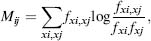

where f_xi, f_xj is the frequency of each four bases in column i and j respectively, and f_xi,_xj is the frequency of the 16 possible pairs observed in i and j.

Two conditions must be satisfied for a helix to be predicted using phylogenetic analysis. First, the complementary sequences of a helix must occur in homologous parts of the multiple sequences. Second, two or more independent covariations must occur in the complementary sequences in such a way that the base pairing is preserved. Although only canonical (A/U, G/C) pairs are considered initially, noncanonical pairs (e.g., G/U) can be considered after a helical region has been determined.

When enough sequences are available, covariation analysis is considered the gold standard for secondary structure prediction methods with successful application to many families of RNA, including 5S RNA (Fox and Woese, 1975) and rRNAs (Woese et al., 1983). The multiple sequence alignments and covariance models used in these predictions can be found in several databases such as Rfam built by Griffiths-Jones and coworkers that currently contains 574 families (Griffiths-Jones et al., 2003), and the Comparative RNA Web (CRW) createdby Gutell and coworkers that contains detailed secondary structure models for several RNA families (Cannone et al., 2002). We have included links to these sites at the end of this chapter.

The success of this powerful technique stems from the inherent unrestrictive model-free approach to the prediction of RNA secondary structure, thus allowing predictions of pseudoknots, triple pairs, and even long-range tertiary single pairs. In a 2002 paper, Gutell and coworkers measured the accuracy of secondary structure models predicted by covariation analysis for the 16S and 23S rRNA molecules by comparing them with information from the solved crystal structures. They found that covariation analysis was able to predict all of the standard secondary structure base pairings and helices, as well as some of the tertiary interactions (Gutell, Lee, and Cannone, 2002). However, this method is limited by its need for a family of molecules with 60-80% identity, as well as manual intervention for editing the multiple sequence alignment.

Energy-Based Dynamic Programming Methods

These methods for predicting RNA secondary structure are based on the observation that the stability of a helical region is the ensemble of individual energy contributions from local interactions. To predict secondary structure within a molecule, all the possible helical regions are given an energy score based on their components. Dot plots are a simple approach to finding possible helices by marking all possible base pairs on a two-dimensional grid of the primary sequence versus itself (Jacobson and Zuker, 1993) with diagonal regions revealing potential helix formation. Figure 33.1b shows such a plot for the yeast phenylalanine tRNA with the lower right triangle showing all the possible helices, while the top left triangle shows the helices that are present in the molecule.

Putative helices are given an energy score based on interactions within the helix. The three main interactions that contribute favorably to the stability of a helix are (1) hydrogen bonds of base pairs, (2) stacking interactions between bases, and finally, (3) irregular structures, such as tetraloops at the ends of helices. In addition to these favorable contributions, unfavorable contributions from both asymmetric and symmetric bulges within a helix, large loops at the ends of helices, and multiple branches stemming from a single loop are accounted for in the energy function. Each of these phenomena is assigned an energy contribution, which is added up for each helix to determine its likelihood. Lower energies correlate with more stable helices, whereas a high energy means that the helix is unlikely to exist in the structure (Zuker and Stiegler, 1981).

An example of a simple energy model is to assign the following energy values to base pairs in a potential helix:

G-C = — 3 energy units (this is the most favorable Watson-Crick pairing.)

A-U = —2 energy units

G-U = — 1 energy unit (this is a noncanonical pairing.)

Turner and coworkers enabled more complicated thermodynamic parameters based on experimental measurements to calculate the contribution of each base pair (Xia et al., 1998) and to incorporate position-specific parameters (Mathews et al., 1999). Zuker and coworkers incorporated these parameters into a secondary structure prediction tool called Mfold (Zuker and Stiegler, 1981), which is now available online as a web server (Mathews et al., 1999; Zuker, 2003). Instead of generating all the possible helices using the dot plot method described earlier, Mfold uses a dynamic programming approach that calculates the lowest free energy for each possible sequence fragment, starting with the shortest fragment. This method uses a recursion on the determined energies of smaller fragments to calculate free energies of longer fragments. Other popular energy-based secondary structure prediction programs include RNAfold and RNAstructure, which are also based on dynamic programming algorithms.

Energy-based methods are limited by the quality of their parameters. Furthermore, pseudoknot structures are difficult to predict. For example, the effects on stability, such as bulge loops and single noncanonical pairs, are nonnearest-neighbors and are not included in these models (Longfellow, Kierzek, and Turner, 1990; Burkard et al., 1999; Kierzek, Burkard, and Turner, 1999). Energy-based methods assume that RNA sequences are at equilibrium and do not consider the role of folding kinetics in the formation of secondary structure. Moreover, some RNA molecules have more than one secondary structure conformation. For example, ribos-witches can take on different secondary structures in the presence and absence of a metabolite.

To address some of these limitations, energy-based prediction methods now report suboptimal structures since the lowest energy structure may not be the correct (or only) one. For example, Mfold and similar programs calculate both the energetically optimal structure and the diverse set of suboptimal structures that have free energy values similar to the optimal structure (Mathews, 2006).

Unlike the phylogenetic analysis strategy, energy-based methods do not take a model-free approach and assume that helices are well nested and therefore are not able to predict structures such as pseudoknots and triple bases. This is a serious limitation because structured functional RNAs often contain these nonnested structural units. Rivas and Eddy addressed this limitation in 1999 with their dynamic programming algorithm for predicting RNA secondary structure, including pseudoknots, with thermodynamic parameters from energy-based methods (Rivas and Eddy, 1999). However, because it is prohibitively computationally expensive, it can only be used for small RNA molecules.

Grammar-Based Methods

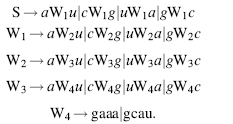
Grammar-based methods examine the palindrome-like primary sequence as a consequence of conserving these base-pairing interactions. This strategy utilizes tools created by research advances in computational linguistics to examine palindrome in languages, in particular the context-free grammars (CFGs) in Chomsky’s hierarchy of transformational grammars (Chomsky, 1956; Chomsky, 1959). These CFGs are developed and used for the specific purpose of predicting RNA secondary structures.

A transformational grammar is made up of symbols and rewriting rules α→β (also called productions) where α and β are both strings of symbols. Symbols may be either nonterminal or terminal, and the left-hand side α must contain at least one nonterminal, which is rewritten into a new string of symbols. Terminals are generally represented with lower case letters, while nonterminals are represented with upper case letters.

To illustrate transformational grammar, we will give an example of a very simple regular grammar that can be used to generate strings of a and b. Regular grammars are the simplest and most restrictive type of grammars, allowing only production rules of the form W → aW or W → a. Using the terminal letters a and b, a single nonterminal letter S, and a blank terminal symbol e, a simple example of a transformational grammar is

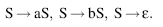
This can also be represented as

This grammar can be used to generate strings of a and b. For example,

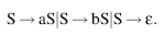
Context-free grammars are the second of the four types of grammars in the Chomsky hierarchy and are slightly less restrictive than regular grammars, which are the first type. Context-free grammars allow any production rule of the form W → β, where the left-hand side must consist of just one nonterminal, but the right-hand side can be any string. This allows the grammar to create nested, long-distance pair-wise correlations between terminal symbols. This type of grammar is appropriate for RNA secondary structure prediction because it can generate RNA primary sequences with nested base pairs. For example, the sequence accggaaacggu, which is an RNA stem with four base pairs and a loop, can be built using the following simple grammar:

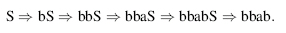
Here is the derivation that results in our example sequence:

Grammar-based methods of RNA secondary structure prediction use stochastic context-free grammars, in which each production rule is assigned a probability. These methods have elaborate production rules and are used to build statistical models of RNA families, perform multiple sequence alignments, and predict secondary structures (Eddy and Durbin, 1994; Sakakibara et al., 1994; Grate, 1995; Lefebvre, 1995; Lefebvre, 1996). Implementations of stochastic context-free grammars, including covariance models, are well covered in Biological Sequence Analysis by Durbin et al. (1998).

Like the energy-based methods described earlier, SCFGs are also unable to handle nonnesting occurrences of base pairs, preventing them from predicting pseudoknots, triple pairs, and long-range interactions.

Genetic Algorithm Approaches

Generally, the genetic algorithm is a stochastic method that uses concepts from evolution and the survival-of-the-fittest individual to find a solution. This algorithm proceeds stepwise and yields a set of probable solutions that it attempts to improve at each step. Each step consists of three procedures:

1. mutation, which introduces random changes into the solutions,

2. crossover, which exchanges parts of solutions with each other, and

3. selection, which uses a fitness criterion to select the best solutions.

Several programs implement the genetic algorithm to solve RNA secondary structures. These include a method by van Batenburg, Gultyaev, and Pleij (1995) and MPGAfold (Shapiro and Navetta, 1994; Shapiro and Wu, 1997; Shapiro et al., 2001). These methods generate initial possible solutions from the set of all possible stems, and allow them to evolve, using free energy as a measure of fitness in each selection step. These methods permit the formation of pseudoknots and are also able to capture significant intermediate RNA secondary structure states, giving insight into the RNA folding process (Shapiro et al., 2001; Kasprzak, Bindewald, and Shapiro, 2005).

Other Approaches

CONTRAfold, a secondary structure prediction tool developed by Do and coworkers, uses a class of probabilistic machine-learning methods called conditional log-linear methods (CLLM). CLLMs are more flexible than SCFGs and allow the incorporation of thermodynamic parameters determined in energy-based methods. By using the strengths of both SCFG and energy-based methods, CONTRAfold is able to outperform both, although it inherits their limitation of not being able to predict nonnested structures such as pseudoknots (Do, Woods, and Batzoglou, 2006).

Several methods incorporate both thermodynamics and covariation data from multiple sequence alignments into RNA secondary structure predictions. These methods include iterated loop matching (Ruan, Stormo, and Zhang, 2004a; Ruan, Stormo, and Zhang, 2004b), KNetFold (Bindewald and Shapiro, 2006;Bindewald, Schneider, and Shapiro, 2006) and HXMATCH (Hofacker, Fekete, and Stadler, 2002; Witwer, Hofacker, and Stadler, 2004). These methods generally start with pseudoknot-free structures, but are able to make predictions that include pseudoknots by combining thermodynamics with covariation data. These methods are reviewed and described in greater detail in Shapiro et al. (2007).

Several other successful methods include Kinefold, a web server that implements stochastic folding simulations using a Monte Carlo methodology (Xayaphoummine et al., 2003; Xayaphoummine, Bucher, and Isambert, 2005) and HotKnots, a heuristic approach that iteratively forms stable stems (Ren et al., 2005). Both of these methods allow alternative secondary structures to form and are able to predict pseudoknots.

THREE-DIMENSIONAL MODELING METHODOLOGY

RNA Motifs

By studying RNA crystal structures, researchers have identified and characterized numerous RNA secondary and tertiary structure motifs: recurring structural building blocks from which RNA molecules are built. When the crystal structures of the large and small subunits of the ribosome were solved, researchers found them to be mostly made up of known RNA structural elements. Motifs are classically defined and described as a pattern of interactions between elements of RNA structure. Motifs consistently fold into the same 3D structure, and the formation of these motifs affects both the folding and the final structure of RNA molecules by facilitating the formation of additional contacts such as hydrogen bonds between backbones, bases, and backbones and bases (Lescoute et al., 2005; Leontis, Lescoute, and Westhof, 2006).

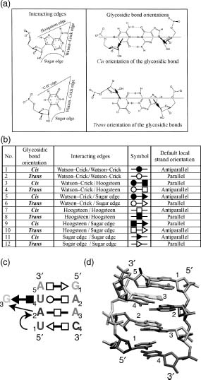
RNA motifs are often the result of non-Watson-Crick base pairing. In addition to the classical Watson-Crick base pairing described in Chapter 3, there are additional families of base-base interactions frequently found in RNA structures. Figure 33.2a shows the three interacting edges of a base, Hoogsteen, Watson-Crick, and sugar, as well as the two relative bond orientations, cis and trans. Figure 33.2 lists the 12 geometric families of edge-to-edge base pairs. Figure 33.2c shows an example of a symbolic representation of the sarcin motif. Figure 33.2d shows the three-dimsensional structure of the sarcin motif found in the 23S rRNA of H. marismortui (Leontis, Stombaugh, and Westhof, 2002b; Leontis and Westhof 2003).

A number of tools search through RNA sequences for known motifs. One of these, the RNAMotif tool, translates a motif into a search tree based on nesting within the motif, and then performs a depth first search to find motifs within a sequence (Macke et al., 2001). Some motif search tools use information from high-quality secondary structure predictions that include non-Watson-Crick base pairs. These methods use the predicted secondary structure to identify potential regions for motifs and check them against known consensus motifs (Leontis, Stombaugh, and Westhof, 2002a). A review by Holbrook from 2005 lists occurrences of known RNA motifs in solved RNA structures, as well as novel motifs found in each structure (Holbrook, 2005).

Constraint Satisfaction

The program MC-SYM (Macromolecular Conformation by SYMbolic generation) written by Major and coworkers in 1991 can produce atomic resolution three-dimensional models of RNA molecules (Major et al., 1991). The inputs to this program are a sequence of nucleotides and their relationships, such as base pairing, and a set of constraints, such as distances between specified residues.

MC-SYM uses a constraint satisfaction problem (CSP) algorithm to model RNA structures at the atomic resolution. A CSP algorithm looks for values of X = {x₁, x₂ ... x_n} that satisfy a set of constraints C = {c_p,q, | p ∈ {1 ...n}, q ∈ {1 ...p — 1}}, where the values of X are taken from a set of allowed values D = {d₁, d₂ ... d_n}. In the application to RNA structure, the values of X are the atomic coordinates of nucleotides 1 through n. The constraints in C are relationships between nucleotides such as base pairing or stacking. The set of allowed values D for the geometry of each nucleotide was chosen from a limited set of internucleotide and internal nucleotide torsion angles found in the crystal structures of tRNA molecules. Relationships between pairs of nucleotides are indicated by the user and determine the set of allowed geometries. These relationships include free connections, stacked connections, Watson-Crick and reverse Hoogsteen base pairs, and A-helix form. For a free connection to the 3’ end of another nucleotide, there are 10 combinations of the four internal torsion angles α, β, δ, and χ, combined with three torsions of the internucleotide bond ζ, resulting in 30 possible geometries of a nucleotide (refer to Figure 3.2 in Chapter 3 for locations of torsion angles).

The CSP algorithm generates a search tree, where each node corresponds to the assignment of a geometry to a nucleotide. The program evaluates the consistency of each assignment with the constraints, and continues with the next assignment if the constraints are satisfied. If the constraints are not satisfied, the program backtracks by removing the current node and its branches, returning to the previous node. The result of this method is a set of possible geometries for the given sequence of nucleotides and their interactions and constraints. This method does not directly prevent the overlapping of atoms, so a round of energy minimizations, which can remove these collisions, usually follows it.

This method does very well with small RNA structures such as the motifs discussed in this chapter. It has successfully predicted loops and pseudoknots to within 2.0-3.0 Å RMSd to the known or consensus structures. In addition, MC-SYM generated full atomic structures of RNA substructures such as hairpin loops that can be used as building blocks for modeling larger structures. In 1993, Gautheret and coworkers used MC-SYM to generate full atomic models of the tRNA T-loop, UUCG tetraloop, tRNA anticodon, and hairpin loops (Gautheret, Major, and Cedergren, 1993). Major and coworkers then used these substructure models to build a full atomic model of tRNA (Major, Gautheret, and Cedergren, 1993).

Altman and coworkers have also used a constraint satisfaction method to produce a model of the 16S ribosomal RNA subunit (Altman, Weiser, and Noller, 1994). Constraints were based mostly on chemical probing results. Furthermore, an analysis of the structural information content of the different experimental modalities used in these models was carried out after the ribosomal structure was solved by X-ray crystallography (Whirl-Carrillo et al., 2002).

Fragment Assembly of 3D RNA Structures

Tools that model large RNA structures generally treat RNA molecules as assemblies of smaller fragments. These tools use known structures of small RNA fragments and require user interaction to assemble them into larger structures.

The MANIP tool allows a user to assemble an RNA structure from a set of smaller RNA fragments (Massire and Westhof, 1998). MANIP uses a database of known fragment structures, assembled from RNA structures solved by NMR or X-ray crystallography. MANIP begins its modeling process by refining the molecule’s secondary structure using an alignment of available RNA sequences. MANIP then recognizes structure motifs within the secondary structure and constructs these fragments automatically based on the database of known fragment structures. MANIP then assembles these fragments and integrates available experimental data. The program NUCLIN/NUCLSQ further refines the resulting structure. This tool has successfully modeled the RNAse P molecule (Massire and Westhof, 1998; Tsai et al., 2003).

Another interactive tool for modeling large RNA structures is ERNA-3D, which produces 3D representations of molecules from known secondary structures, using knowledge of motif structures from other RNAs (Zwieb and Muller, 1997). This tool allows a user to manipulate the 3D-motif structures and position them manually. This tool was used to build a high-resolution 3D model of several transfer-messenger RNAs (Burks et al., 2005).

Other 3D Modeling Tools

The Nucleic Acid Builder (NAB) is a computer language developed to construct models of nucleic acids up to a few hundred residues in size (Macke and Case, 1998). This tool uses a combination of rigid body transformations and distance geometry to generate structures that are then refined by molecular dynamics. The RNA2D3D program can generate, view, and compare 3D RNA structures as well as generate a first-order approximation of a small RNA molecule or fragment of a molecule. This tool has been used to predict the 3D structure of a pseudoknot (Yingling and Shapiro, 2006). Finally, S2S is a tool that links several levels of RNA data, including multiple sequence alignments, secondary structure, and tertiary structure (Jossinet and Westhof, 2005).

CONCLUSION

The RNA world is rich with computational opportunities both at the 2D and 3D levels. The unique chemical nature of the RNA sugar-phosphate, combined with the base-pairing promiscuity yields a highly complex biopolymer that plays a critical role in the cell. As the multifaceted roles of RNA in the cell become more apparent, computational approaches that assist the biological community in deciphering these roles will be critical.

WEB RESOURCES

RNA World Website	http://www.imb-jena.de/RNA.html
Functional RNA database	http://www.ncrna.org/
Rfam database of RNA alignments and covariance models	http://rfam.janelia.org
Comparative RNA Web	http://www.rna.ccbb.utexas.edu
Mfold web server	http://www.bioinfo.rpi.edu/applications/mfold/

SUGGESTED READINGS

1. Secondary structure prediction methods:

• Chapter 8 of Bioinformatics: Sequence and Genome Analysis by David W. Mount (Mount, 2004).
• Chapters 9 and 10 of Biological Sequence Analysis by R. Durbin, S. Eddy, A. Krogh, and G. Mitchison (Durbin et al., 1998).

2. An excellent review on RNA structure prediction:

• A 2007 review by Shapiro and coworkers on RNA structure prediction: bridging the gap in RNA structure prediction (Shapiro et al., 2007).