37
PROTEIN MOTION: SIMULATION
“If we walk far enough,” said Dorothy, “we shall some time come to some place, I am sure.”
L. Frank Baum, in The Wonderful Wizard of Oz, 1900.
INTRODUCTION
Molecular motions of biological macromolecules underlie folding, stability, and function. Crystallographic structural snapshots (Chapter 4) as well as nuclear magnetic resonance (NMR) structural (Chapter 5) ensembles enable, with the help of bioinformatics methods, the identification of functional sites, hinge and dynamic regions, interacting partners, remote homologues, and much more valuable biophysical insights. Yet, this experimental structural view is often constrained by the lack of understanding of the underlying time-dependent mechanism bridging structure and the execution of biological function. Understanding protein motion is pivotal for deciphering functional mechanisms including folding (Daggett and Fersht, 2003; Vendruscolo and Paci, 2003; Munoz, 2007) along with the complimentary misfolding (Dobson, 2003; Chiti and Dobson, 2006; Daggett, 2006), allosteric regulation (Popovych et al., 2006; Swain and Gierasch, 2006; Gilchrist, 2007; Gu and Bourne, 2007), catalysis (Hammes-Schiffer and Benkovic, 2006), functional plasticity (Kobilka and Deupi, 2007), protein-DNA interactions (Sarai and Kono, 2005), and protein-protein interactions (Bonvin, 2006; Fernandez-Ballester and Serrano, 2006; Reichmannet al., 2007). While information from different static structures can be morphed yielding a dynamic path between the structures (Flores et al., 2006), it is often required to simulate a static structure or substructure in a time-dependent manner in order to provide a dynamic understanding.
Simulating protein motions began in 1969 with the first energy minimization of proteins using a general force field (FF; Levitt and Lifson, 1969). In this study, Levitt and Lifson applied 50 steepest descent iterations (described later) to lysozyme and myoglobin. For the small 964-atom lysozyme it took 3 h of computing time on a room-size computer whose name was “Golem.” Interestingly, the semiempirical FF applied in this early work is not much different than today’s classical mechanics common FF. The nontrivial shift from minimization to molecular dynamics (MD) simulation that follow the trajectories of each atom of a protein utilizing classical Newtonian molecular mechanics (MM) was conducted in 1977 by McCammon, Gelin, and Karplus (1977). Their in vacuo MD simulation of the 58-residue bovine pancreatic trypsin inhibitor spanned 9.2 ps (10-12s). It took 11 more years for a full-atom (namely, including hydrogens) simulation of this protein to be carried out in the presence of solvent water (Levitt and Sharon, 1988) molecules to be realized, setting the stage for modern MD protein simulations. This classical approach to describe systems of biological interest provides insight regarding the molecular conformational changes that give rise to the observed functional consequences; and all this in the presence of solvent water and counter ions as appropriate. Today, the most powerful available computers, for example, Blue-Gene, are being utilized for MD simulations, with size, resolution, and time length of the simulations still growing. Actually, the very name “Blue-Gene” was given in 1999 due to the specific aim of this computer to solve the protein folding problem via the simulation of protein motion (IBM, 1999). Indeed, the importance of this theoretical field is reflected by a growing number of publications contributing ~1200 publications on protein MD in 2007 alone (ISI Web of Science query “TS = (protein) and TS = (molecular dynamics)”).
In this chapter we will focus solely on computational methods aimed at understanding protein motion. While most such tools are applicable for other biomacromolecules as well, for example, nucleic acids, we will not dwell into methods tailored for them. MD simulation yields the history of the motion (so-called trajectory) of each atom comprising the protein of interest and can therefore provide us with a microscopic characterization of the system. The conversion of the microscopic information to macroscopic thermodynamic observables, such as pressure, energy, heat capacities, and so on, requires statistical mechanics. The ergodic hypothesis (Chapter 8) enables the derivation of general conclusions on the system from a sufficiently long MD simulation of a protein molecule. Briefly, the hypothesis claims that a large number of observations made on a single system at many arbitrary instances in time have the same statistical properties as observing many systems, arbitrarily chosen from the phase space at one time point. One of the key challenges of a proper MD simulation of protein motion is the design of a time-dependent simulation that will obey ergodicity. One of the methods to assess whether the system indeed obeys ergodicity is to conduct multiple MD runs and thereby assess convergence. As demonstrated by the Blue-Gene team by analyzing 26 independent 100 ns MD runs of rhodopsin, much care should be applied when assuming ergodicity of a single trajectory (Grossfield, Feller, and Pitman, 2007). The challenge includes two aspects-what is a “sufficiently long” time and how can we ensure that the “relevant” phase space was indeed fully investigated (sampled). Notably, the latter aspect requires the nontrivial definition of a relevant phase space. Most often, not all phase space is of interest but only the low-energy wells within the complex (rugged) energy landscape of the system that are involved in executing the biological function. The movement between energy wells is specifically challenging, as on the one hand small time steps are needed to follow high-frequency motions of light atoms like hydrogen whereas on the other hand, long time (many time steps) is required in order to grasp transitions that underlie the slow timescale motions of protein domains undergoing conformational changes (Figure 37.1). In order to solve these challenges, different resolutions of physical properties and time steps are used to address macromolecular motion occurring at different timescales.
The study of molecular motion via computational methods has advanced to a state where there are many resources available to a wider scientific community. Understanding protein motion has been an important research field in itself and will become increasingly recognized in the field of structural bioinformatics since protein flexibility and dynamics is inextricably linked to its function. The importance is exemplified by new databases such as ProMode (Wako, Kato, and Endo, 2004) containing a collection of NMA simulations and MolMovDB (Flores et al., 2006) containing extrapolated motion as well as simulations for single structures. These resources allow researchers to appreciate the full range of protein motion diversity and will continue to become of growing utility to the community (Gerstein and Echols, 2004). More importantly, these databases set a foundation in which to develop an improved systematic approach to categorize and expand our understanding of protein motion in a large-scale fashion as more structures become available to study the function and dynamics of biomolecules.
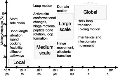
Figure 37.1. Characteristic division of protein motion to time and amplitude scales (division after Becker (2001)). This schematic division isconvenientfor motion analysisand simulation. In reality, the timescale and amplitude of many of the described phenomena are far more disperse. For example, some allosteric transition may take up to a second or alternatively, helix-coil transitions may initiate in the submicrosecond time regime. Designed, self-folding mini-proteins fold on the fast microsecond timescale (Bunagan et al., 2006). Other movements highly depend on local environment; for example, side-chain rotation istypically quick when solvent exposed (10_11-10-10s) and slow when buried (10-4-1 s). The timescale division is also relevant from the aspect of disorder (Chapter 38).
Many of the off-the-shelf packages can be operated without requiring deep fundamental understanding of the underlying theory. Yet, it is important to have a basic appreciation for the theory behind the different techniques in order to receive correct results and in order to correctly interpret the results. Rather than providing an exhaustive compilation of resources available to the community and rather than providing thorough mathematical foundations, this chapter aims to provide a brief introduction to the fundamental terms and theoretical rationale behind computational approaches aimed at understanding protein motion. The differences between various simulation approaches, along with their applicative strengths and limitations for interpretation, will be highlighted. For further understanding of this established yet evolving field, readers are referred to recent textbooks (Becker, 2001; Leach, 2001; Schlick, 2002; Cui and Bahar, 2006; Holtje, 2008), meetings lecture notes (Leimkuhler, 2006), as well as reviews on biomolecular simulation in general (Norberg and Nilsson, 2003; Schleif, 2004; Jorgensen and Tirado-Rives, 2005; Karplus and Kuriyan, 2005; Adcock and McCammon, 2006;Scheraga, Khalili, and Liwo, 2007). Several reviews cover specific aspects of the methodology such as long time-scale simulations (Elber, 2005), coarse-grained models (Tozzini, 2005; Levy and Onuchic, 2006), and so-called QM-MM methods (Friesner and Guallar, 2005; Dal Peraro et al., 2007a; Senn and Thiel, 2007). Other reviews focus on MD simulation utilized for specific applications such as membrane and membrane-protein simulations (Saiz and Klein, 2002; Roux and Schulten, 2004; Gumbart et al., 2005;Brannigan, Lin, and Brown, 2006; Feller, 2007;Kandt, Ash, and Tielman, 2007; Lindahl and Sansom, 2008), steered MD applications (Sotomayor and Schulten, 2007), drug design (Alonso, Bliznyuk, and Gready, 2006), and adaptation to extremophile conditions (Tehei and Zaccai, 2005).
PROTEIN MOTION TIMESCALES, SIZE, AND SIMULATION
The structural changes underlying protein motions occur on timescales ranging over several orders of magnitude (Figure 37.1). Each timescale range contributes to different biophysical aspects of the protein. The complimentary biophysical forces involved in different types of motion scales can be batched according to their resolution and extent of affect they have on the motion. The very existence of a wide range of timescales is a major component of the multidimensional complexity that has to be addressed when studying protein motion. Intrinsic to this complexity is the manner in which the different types of motions are coupled. For example, the allosteric R to T transition of hemoglobin takes tens of microseconds to complete. This major change requires the relaxation of the heme cofactor (picosecond range), tertiary structure relaxation (nanosecond range), and so forth.
The relationship between theoretical and experimental study of protein motion is not limited to cross-validation but expands to the very parameterization of the many knowledge-based theoretical methods. On the experimental side, a wide plethora of biophysical spectroscopic methods are tailored to explore motions of different scales. Hydrogen deuterium exchange explored via NMR (Krishna et al., 2004) and via mass spectroscopy (Tsutsui and Wintrode, 2007; and Chapter 7), time-resolved Förster (commonly replaced by the word “fluorescence”) resonance energy transfer (FRET) (Förster, 1948), laser-induced temperature jumps (Hofrichter, 2001), site-directed spin labeling (Fanucci and Cafiso, 2006), and time-resolved crystallography (Moffat, 2001) are just a few of the common methods used to study the kinetic aspect of protein motion. Other methods were developed to study thermodynamic aspects such as barrier heights and the corresponding free energy associated with specific types of motions. Similarly, a large number of distinct computational methods were developed to study different timescales of computational motions. The gaps between the complimentary experimental and theoretical methods are closing with an increasing degree of supporting cross-referencing, for example, as reviewed for the study of protein folding (Vendruscolo and Paci, 2003).
Ideally, all motion studies should account for all the physical forces of the system and the surrounding solvent when simulating the fastest identified discrete movement. However, solving the full Schrodinger equation is too complex and approximations are embedded, even in quantum mechanical (QM) calculations. In addition, as the time evolution of each computed variable is affected by many other variables, the complexity of the computation scales exponentially with the size of the studied system. Nontrivial challenges also arise with the definition of the basic time unit to be simulated and the distance after which the effect of the surrounding forces can be neglected. Lastly, the basic time-step unit that can be stably integrated should be considered. As shown in Figure 37.1, such a time step should be around 1 fs giving rise to intractable computation time for slow processes of the large biomacro-molecules. Consequently, simulations of macromolecules represented at different resolutions are used for the study of motions of different timescales. As such, alternative approaches involving a reduced or more detailed representation of protein structures have been developed (Figure 37.2).
Figure 37.2. The features of bead models. Schematic representation of the model, indicative number of parameters, methods of solution, main characteristics, and applications are shown for each model. Sample applications are also illustrated with representative pictures (PDB codes 1HHP, 1CWP, 1MWR, 486D) showing the size of a studied system and the kind of study that can be done. The location of the models in the x-y plane qualitatively illustrates their complexity in system size (x-axis) and parameterization (y-axis). Reprinted with permission from Tozzini, 2005.

Protein motion is studied utilizing methods ranging from detailed QM to coarse-grained models. The main driving force to the development of these models is to circumvent issues arising from computational demands resulting in the intractability of simulating very large biomolecules coupled to the varying demands of resolution requested from the simulation. Resolution includes the size of the system involved in the motion, the duration of the motion assessed, and the details of the factors affecting the motion. Different aspects of the resolution challenge are addressed by different approaches. For example, often the area of prime interest is a very small segment within the full system. Consequently, several simulation methods enable a differential resolution of different regions of the system. These include modeling the atoms of the macromolecule explicitly while modeling the solvent implicitly. In this context, the very term “explicitly” has different meanings in different motion simulation subfields: The classical FF (Figure 37.3) is considered explicit when compared to implicit solvent. However, while using QM-MM methods to investigate enzyme catalysis, the area of prime interest, for example, the active site, is modeled explicitly via QM methods and the rest of the system (protein and solvent) is described with classical MM.
Figure 37.3. Common force field (FF) energy function components exemplified on a Phe-Ala dipeptide. Cross-terms such as Urey-Bradley and improper out-of-plane terms are part of higher order force fields. The external energy Coulombic electrostatic term and van der Waals Lennard-Jones terms are shown here for a sodium ion but, like all other depicted terms, are computed for all relevant atoms. Likewise, the out of plane improper term can be described for any group of three or more atoms and not only for aromatic rings. Elements such as lone pairs can be described via “extended point” pseudoatoms or by adding polarizability to the FF.

As MD simulations yield a trajectory of the motion, it is appealing to data mine this “movie” with every relevant bioinformatics approach. Yet, it is pivotal to fit the resolution of the analysis and conclusions to the resolution of the data. In this chapter the computational study of motion is presented in a top-down approach. The presentation of the coarse-grained methods will be followed by MM approaches, which in turn will be followed by QM-MM methods. Thus, each section will give insight on the resolution-related limitations of the previous section.
COARSE-GRAINED METHODS
As suggested in Figure 37.2, slow and large movements are often sufficiently hard-wired into the protein to be well represented by the use of a reduced coarse-grained representation of the structure (Tozzini, 2005; Levy and Onuchic, 2006). Alternatively, it can be stated that groups of adjacent atoms, for example, residues, move sufficiently in concert to be parameterized as a single point in space. Complementary, the expansion of motion simulation into the mesoscale (microsecond) time regime as well as into large interacting protein-protein complexes can be facilitated by coarse graining. In MD simulations, coarse-grained models are gaining increased attention. As not all atoms contribute similarly to the assessed question, the coarse graining can focus on the less significant atoms, for example, solvent and nonpolar hydrogens. The exclusion of nonpolar hydrogens, referred to as united atom FFs, “unifies” the hydrogen’s additional mass and movement constraint into the atom to which it is attached forming a larger pseudoatom. The united atom approach is especially meaningful for membrane proteins where a large portion of the simulation computes the nonpolar bilayer.
The reduced representation of the structural space, also termed a bead- or minimalist-model, can be applied in several levels. Intuitively, each residue can be represented by a single bead, typically modeled at the coordinates of the Cα central atom. To get a better appreciation to the protein structure and without a large computational increase, a representation of the Cβ atom (Micheletti, Carloni, and Maritan, 2004) or centroid pseudoatoms representing a group of atoms with similar properties, for example, side-chains (Becker et al., 2004) or atom groups within a lipid (Saiz and Klein, 2002; Marrink et al., 2007; Saiz et al., 2002), may be embedded. Another important coarse-graining approach includes a differential resolution of different parts of the simulated system. Most broadly, this includes applying a hierarchy of up to four different resolutions of simulations: (a) simulating the active site of an enzyme with a high-resolution (in this case electrons) QM scheme, (b) embedding the active site within a segment of the protein framework treated via a classical Newtonian dynamics and an empirical interatomic FF, (c) linking the protein segment to a coarse-grained treatment of the protein framework, and (d) representing the solvent implicitly. These applications are discussed in the relevant sections below.
Coarse graining of the protein model can vary also in the type and character of the
connectors modeled between the beads. Thirty years ago, Go and coworkers studied folding via placing
repulsive and attractive connectors representing nonbonded interactions between the one-residue beads
(Ueda, Taketomi, and G , 1978). The
resulting G models reproduce several aspects
of the thermodynamics and kinetics of folding, largely due to the fact that the folding process has
generally evolved to satisfy the principle of minimal frustration (Baker, 2000). The minimal frustration principle states that naturally occurring proteins have
been evolutionarily designed to have sequences that achieve efficient folding to a structurally
organized ensemble of structures with few traps arising from discordant energetic signals. Frustration,
for example, via solvation terms, can be added to the model in order to roughen the energy surface,
enabling the appearance of stable intermediate states. As reviewed by Levy and Onuchic, the complexity
and character of minimalist models can be tailored to the question addressed, for example the detailed
assembly mechanism of aprotein complex (Levy
and Onuchic, 2006). Notably, enhanced connectivity may be applied between interacting regions or
electrostatics may be represented by providing different parameterization such as beads representing
charged amino acids (Levy and Onuchic, 2006).
, 1978). The
resulting G models reproduce several aspects
of the thermodynamics and kinetics of folding, largely due to the fact that the folding process has
generally evolved to satisfy the principle of minimal frustration (Baker, 2000). The minimal frustration principle states that naturally occurring proteins have
been evolutionarily designed to have sequences that achieve efficient folding to a structurally
organized ensemble of structures with few traps arising from discordant energetic signals. Frustration,
for example, via solvation terms, can be added to the model in order to roughen the energy surface,
enabling the appearance of stable intermediate states. As reviewed by Levy and Onuchic, the complexity
and character of minimalist models can be tailored to the question addressed, for example the detailed
assembly mechanism of aprotein complex (Levy
and Onuchic, 2006). Notably, enhanced connectivity may be applied between interacting regions or
electrostatics may be represented by providing different parameterization such as beads representing
charged amino acids (Levy and Onuchic, 2006).
As functional motions of proteins are usually cooperative and include fluctuations around native states, normal mode analysis (NMA) methods are well fit to gain insight into these important dynamics. This topic is often viewed as part of the coarse-grained dynamic description via an elastic network models (ENMs), which is often sufficient to achieve valuable results. Although normal modes do not provide a fully detailed motion trajectory, they do yield the direction and relative magnitude of movement of regions within the protein. While here we focus on ENM-related methods, it is important to remember that normal modes are a more general framework frequently utilized as an analysis tool to understand dynamical trajectories of proteins produced by other types of simulation methods.
By definition, NMA is the study of harmonic potential wells by analytical means. NMA is the
most direct quick way to obtain large amplitude, low-frequency motions (G , 1978; Brooks and Karplus, 1983). This rapidly growing
field is maturing into a standard toolbox for the analysis of macromolecular motion (Cui and Bahar,
2006). It is assumed that the energy surface near the minimum can be approximated using a
multidimensional parabola (assumption of harmonic dynamics) that is characterized by the
second-derivative matrix (the Hessian). Solutions to such a system are vectors of periodic functions
(normal modes) vibrating in unison at the characteristic frequency of the mode. Consequently, it is
important that the protein structure is minimized to a single energetic minimum before a simulation is
initiated. The most important distinction from MD simulations is that all variants of NMA approaches
assume that the protein fluctuation is sufficiently described by harmonic dynamics. In other words,
while MD simulations use (a relatively) exact description of the forces between atoms and solve these
equations in an approximate manner, NMA uses approximate equations for motion that can be solved in a
precise manner.
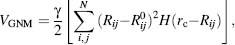
The use of a “single parameter model” for NMA by Tirion (1996) has opened the door for the expansion of more drastically simplified energy potentials used by the ENM approach. The ENM maintains the structures as springs between adjacent atoms, or atom-group centers, consistent with their solid-like nature. Tirion applied a full atom NMA with a uniform harmonic potential. Bahar and coworkers introduced a simplified ENM method termed the Gaussian network model (GNM) to study the contribution of topological constraints on the collective protein dynamics (Bahar, Atilgan, and Erman, 1997). GNM uses the Ca carbon acting as nodes in this polymer network theory undergoing a Gaussian distributed fluctuation. The fluctuation is influenced by neighboring residues typically within a 7 Å distance (rc). The connectivity (or Kirchoff) matrix of interresidue contacts is defined by
(37.1)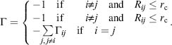
Notably, the diagonal elements of the matrix are equal to the residue connectivity number, namely the degree of elastic nodes in graph theory. This measure is in essence the local packing density around each residue. The contacts are assumed to have a spring-like behavior with a uniform force constant that has been established by fitting to experimental data. Thus, the potential of GNM is given by
where γ is the uniform force constant taken for all springs and  and Rij are the distance vectors between
residues i and j in equilibrium and after a
fluctuation, respectively. This dot product is calculated only for the distances defined by the Kirchoff
matrix as defined by H (rc – Rij), a step function that equals 1 if the
argument is positive and 0 otherwise.
and Rij are the distance vectors between
residues i and j in equilibrium and after a
fluctuation, respectively. This dot product is calculated only for the distances defined by the Kirchoff
matrix as defined by H (rc – Rij), a step function that equals 1 if the
argument is positive and 0 otherwise.
In GNM, the probability distribution of all fluctuations is isotropic and Gaussian.
Alternatively, GNM was extended to the anisotropic network model (ANM) (exemplified in Figure 37.4 insert B; Atilgan et
al., 2001). The potential of ANM is equivalent to that of GNM (Eq. 37.2) except that in ANM and Rij are scalar distances rather than
vectors. For ANM, the scalar product results in anisotropic fluctuations upon taking the second
derivatives of the potential with respect to the displacements along the X-, Y-, and Z-axes. Physically,
in the GNM potential, any change in the direction of the interresidue vector is resisted, that is, penalized. On the contrary, the
ANM potential is dependent upon the magnitude of the interresidue distances without penalizing for
orientation changes. Due to the role of orientation deformations, ANM gives rise to excessively high
fluctuations when compared to the GNM or experimental results. Due to this lower accuracy of ANM, a
higher cutoff distance for interactions is required and the prediction of local relative degrees of
flexibility may be less accurate. Yet, ANM is superior for assessing the directional mechanism of
motion. Since the Kirchhoff matrix is of size of 3N x 3N for ANM compared to N xN
for GNM, GNM is more applicable for supramo-lecular structure analysis.
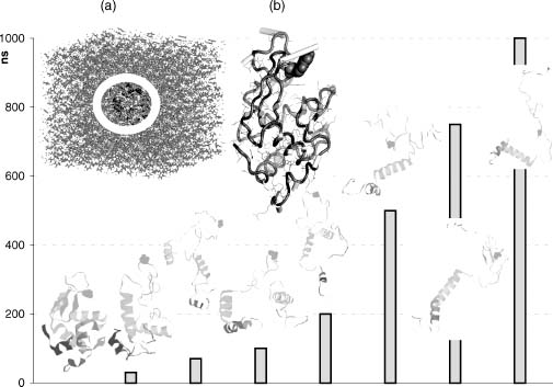
Figure 37.4. Example of a MD simulation. A mutant lysozyme (Trp-62-Gly—residue presented by spacefill) exhibits misfolding along a 1 μs(y-axis, time in nanoseconds) MD simulation trajectory. Snapshots of the protein structures are displayed as the simulation progresses (bars denoting time of each snapshot). The room temperature simulation mimics experimental conditions (Klein-Seetharaman, 2002), for example, 8 M urea (insert A: water box with urea presented via sticks and protein circled) and provide atomic resolution dynamic insight into the role of the mutated residue as a key nucleation site. As the second mode of an ANM standard simulation shows (insert B), different regions around this site move toward different directions (vectors represented by sticks with stick length corresponding to the motion amplitude). In the misfolding simulations some tertiary structure contacts disassemble rapidly while part of the secondary structure remains stable throughout the simulation. Simulation box and trajectory snapshots modified with permission after (Zhou 2007). ANM simulation of the wild-type structure conducted using (Eyal, Yang, andBahar, 2006).
The reproduction of the intrinsic thermal fluctuations within crystal structures (Debye-Waller B-factors) as well as NMR relaxation measurements and H/D exchange free energies provide substantial validation to the ENM approach. Indeed, in recent years, the field of NMA has established itself as a key method for studying protein motion with validation extending comparison to MD studies and numerous other known functional movements, for example, allosteric transitions (Bahar and Rader, 2005; Elber, 2005; Tozzini, 2005; Cui and Bahar, 2006). Interestingly, Gerstein and coworkers have shown that over half of the 38jj known protein motions (inferred from different conformations of the same protein as analyzed from the Database of Macromolecular Movements http://molmovdb.org/) can be approximated by perturbing the original structures along the direction of their two lowest frequency normal modes (Krebs et al., 2002). In addition, the concerted motion of atom groups can be utilized for domain identification or to refine low-resolution models (Ma, 2006). Alternatively, applying NMA on the same domain in different conformations, for example, closed versus open ion channels, enables one to quickly infer a dynamic view of possible pathways between the conformations. Using such an approach as well as benefiting from the ease of applying NMA to nonprotein moieties, Vemparala, Domene, and Klein (2008) recently assessed the interactions of anesthetics with the open and closed conformations of a potassium channel. As a generality, the simplicity of the reduced representation is directly correlated to the smoothing of the local energy surface roughness. The success of the method exemplifies that motion under near native-state conditions is often simple and robust, dominated by the interresidue contact topology of the folded state.
Finally, in addition to traditional molecular simulation techniques strongly rooted in biophysics, the growing availability of structures have provided an alternative and less computationally intensive approach to globally address motion used across different proteins. Proteins solved in multiple conformations has allowed for the inference of biomolecular motion by restrained extrapolation between different structures serving as end points (Krebs and Gerstein, 2000) and is collected in the Database of Molecular Motions (MolMovDB) (Gerstein and Krebs, 1998; Flores et al., 2006). The database framework allows for the construction of a hierarchical categorization for biomolecular movements and the development of a systematic nomenclature for protein motion. First, protein motions are categorized based on molecular size of the biomolecule and the basis of packing that leads to subsequent categorization into the types of motion such as shear and hinge. Categorization based on protein size distinguishes between movements of subunits, domains, and fragments. This resource also contains references to supporting experimental evidence of the extrapolated motions when available. More importantly, it presents a survey of putative protein motions that are available in the “mechanistic toolbox” used by Nature rather than an isolated case interpretation of motion that is modeled in high resolution for a specific system. Hence, the survey allows for bioinformatics-derived interpretations to gain insight and possibly identify new generalized or fundamental rules governing protein dynamics.
CLASSICAL MOLECULAR MECHANICS
System Representation and Energy Function
A prerequisite to the actual time-dependent classical macromolecular motion simulation is the construction of (a) a system for simulation, and (b) a FF that will include the parameters of the system components along with an energy function to compute the system’s energy. In doing so, the contradictory demands for accurate description along with computational efficiency should be addressed.
One of the most critical factors in a time-dependent simulation is the choice of a proper energy function. In classical MM dynamics, hereafter termed MD (except for the QM-MM section) a pseudoempirical potential energy function is utilized. Rather than first principles, additive knowledge-based terms are utilized in the context of the Newtonian laws of mechanics. These constrain the structure to the native form while properly representing the energy required for distorting the structure (Figure 37.3) within the natural range of fluctuations. The potential energy includes additive terms for the “internal” intramolecular energy between covalently bonded atoms and the “external” intermolecular energy found among nonbonded interactions that is
(37.3)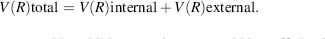
Ideally, each component and its additive constituents would be sufficiently accurate to be analyzed separately. Yet, in the current state of simulation research, the parameterization and resulting fit of the full function to experimental data is the most accurate. Consequently, cross-FF comparison of discrete components of the energy function is not advised. Still, the additive nature of the energy function implies separability, enabling to simulate each part of the function in different time steps (termed “multiple time step dynamics” see section below).
Focusing on a computationally efficient mathematical representation, the internal energy is modeled via a set of springs capturing the bond, angle and dihedral angles:
(37.4)
The b0, θ0, and χ represent the ideal reference parameters for the bond distance, angle, and dihedral angle respectively. For each such term the respective “K” represents the spring constant. The reference parameters of each atom depend on the hybridization, for example, sp2 versus sp3, as well as on the immediate environment such as, aromaticity and electronegativity of adjacent groups. Consequently, FFs include many atom types for each atom depending on the immediate surrounding and chemical nature. As an example, there are over 20 types of carbons.
Equation 37.5 contains the most basic terms but other equations are also in use, for example, bond vibrations are better represented by a double-exponential Morse function. Harmonic bond stretching terms and anharmonic cubic and quartic terms can be used to then reproduce the Morse function potential via a Taylor expansion. The accuracy of bond extension is important for small molecules resulting in the use of such methods in FFs attempting to focus on small molecules, for example, MM4 (Allinger, Chen, and Lii, 1996) and MMFF (Halgren, 1996).
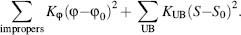
Two additional constraining forces are often added: first, the Urey-Bradley (UB) cross-term represents the distance between two atoms connected through a third atom--the 1 -3 distance corresponding to the angle, namely, the stretch-bend cross-term. Other cross-terms between stretching, bending, and dihedrals are used, especially in FFs focusing on small molecules. Second, the so-called “improper” term aims at fitting computational results with observable vibrational spectra. Unlike the other terms, the improper term is used solely for some of the atoms, for example, improving out-of-plane distortions associated with planar groups—in-plane scissoring and rocking and out-of-plane wagging and twisting. As with the bond and angle terms, these components are modeled by the classical Hooke law for describing a spring, namely,
The external energy includes the van der Waals and the electrostatic Coulomb contributions:
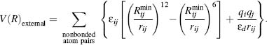
The short-range interatomic repulsion and van der Waals dispersion contributions are
expressed here via the commonly used Lennard-Jones 12-6 potential (Lennard-Jones ,1931). The  represents the rij distance where the Lennard-Jones potential is zero and εij corresponds to the depth of the well found at
the minimum in the energy landscape. Notably, while the attractive exponent is experimentally and
theoretically justifiable, the r-12dependence is
too steep for hydrocarbons but is often used due to the computational simplicity (square of r-6). Consequently, some FFs dampen the repulsive
exponent, for example, down to r-9. Due to the short range of this force, van der Waals forces are computed
only for atoms within a threshold distance.
represents the rij distance where the Lennard-Jones potential is zero and εij corresponds to the depth of the well found at
the minimum in the energy landscape. Notably, while the attractive exponent is experimentally and
theoretically justifiable, the r-12dependence is
too steep for hydrocarbons but is often used due to the computational simplicity (square of r-6). Consequently, some FFs dampen the repulsive
exponent, for example, down to r-9. Due to the short range of this force, van der Waals forces are computed
only for atoms within a threshold distance.
Electrostatics (see also Chapter 24) are represented by Eq. 37.6 using partial charges qi, and qj of the corresponding atoms. The equation is normalized to εd, the effective dielectric constant of the milieu, typically ranging from 2 in membranous environments to 80 in the solvent-exposed regions. The large change between these two numbers is usually conducted using a simple step function. Accurate modeling of the local effective charge density as it gradually changes between different microenvironments is one of the yet unresolved challenges of the field. Assigning partial charges to the many atom groups is a key challenge in constructing the FF. Some FFs were parameterized using a single class of molecules while others, termed “general” FFs, were parameterized using atom groups that should be representative of all the molecules. Thus, one of the main distinctions between FFs is the data set on which it was parameterized and the “transferability” of the parameterization to molecules that are not part of the original data set for which the FF was parameterized. The process of partial charge parameterization, often done via QM methods, is beyond the scope of this introductory chapter. While in the past knowledge-based FFs for specific chemical groups (proteins, nucleic acids, different organomet allo groups) were common, QM-derived parameters of general FFs are becoming more and more accurate. Using a set of molecules that is representative of chemical space, general FFs can be applied to a wide variety of molecules-- a feature that is becoming increasingly relevant for macromolecules subjected to drug design (Chapter 34). In the parameterization process different aspects have to be addressed including the generality and transferability of the parameterization as well as the fit of the partial charge to the condensed phase (rather than vacuum) in which the atom group is expected to be simulated.
The most computationally intensive component within the FF is the electrostatic one because it has the slowest decay with distance and long-range interactions must be included. Beyond the complexity of the function, while the bonded interactions scale linearly, the number of pair interactions scales by N2, with N denoting the number of atoms. Moreover, the electrostatic solute-solvent interactions are important, resulting in much more interactions to compute. Thus, one of the ways to reduce the number of computed atoms is to reduce the number of solvent molecules to a minimum by choosing the correct periodic boundary condition. This condition implies an “image” of the system at the boundaries so a molecule “exiting” the system from one side will “enter” the system from the other side thus avoiding boundary effects. Cubic periodic boundary conditions are mostintuitive to apply and include immersing the solute in a box of solvent (Figure 37.4 A). However, to add efficiency by decreasing the number of computed atoms without loss of accuracy, other conditions are often applied, for example, rhombic dodecahedron or truncated octahedron. For instance, a hexagonal prism may be more appropriate for a long macromolecule such as DNA. Different programs, such as, PBCAID (Qian, Strahs, and Schlick, 2001), can compute the optimal structural periodic domain.
Historically, the Coulomb law was solved using a spherical truncation of the electrostatic interactions conducted in distances in the range of 12 Å. Truncation-based approximation schemes (Seibel, Singh, and Kollman, 1985; van Gunsteren et al., 1986; Miaskiewicz, Osman, and Weinstein, 1993; Steinbach and Brooks, 1994; MacKerell, 1997) are gaining less popularity due to not only the availability of enhanced computing power, but rather the availability of efficient numerical methods. The numerically exact methods include fast multipole methods, which distribute the charge into subcells and then compute the interactions between the subcells by multipole expansion in a hierarchical fashion (Schmidt andLee, 1991). TheEwaldmethod, originally suggested in 1921 (Ewald, 1921), has evolved into a group of increasingly popular methods (Sagui and Darden, 1999). The Ewald summation divides the electrostatic computation to atom pairs within the main cell and those within the reciprocal, periodic boundary cells. The latter are computed using fast Fourier transform. The summation trick includes representing the point charges by Gaussian charge densities, producing an exponentially decaying function that can be summed in the reciprocal space. A correction term is required to ensure the effect of the overall net charges. A major breakthrough, termed particle-mesh Ewald (PME) includes using a grid for a smooth interpolation of the potential for the values in the Fourier series representing the reciprocal state (Darden, York, and Perdersen, 1993). The smoothing interpolation can be applied via Lagrangian (Darden, York, and Pedersen, 1993) or B-spline (Essmann et al., 1995) equations with the latter enabling smoother and more accurate interpolation. Further simplification can be applied by splitting the summation into short- and long-range interactions (Hockney and Eastwood, 1981). The short-range interactions can be computed via direct particle-particle summation while the latter can use the particle-mesh interpolation approach. The resulting particle-particle particle-mesh (Hockney and Eastwood, 1981; P3M) approach is widely used. P3M is easily applicable for parallel computing with specific optimization to parallel systems still evolving (Shaw, 2005).
FFs are available in different resolutions and foci. For example, Scheraga’s ECEPP FF acts in dihedral-angle space (Zimmerman et al., 1977). For Cartesian coordinate FFs the very definition of the basic unit described can vary. The commonly used macromolecular FFs, for example, CHARMM (Brooks et al., 1983), AMBER (Weiner et al., 1984), GROMOS (Vangunsteren and Berendsen, 1977), andOPLS (Jorgensen and Tirado Rives, 1988) include differences in the functional form and in the parameterization. The differences between FFs and the resulting choice of the best FF is a controversial topic that depends on the fit to the specific macromolecule studied, the accuracy requested, as well as individual preferences. In a consensus study aimed to examine what can be inferred about protein MD through the interpretation of these FFs, it was found that some general features are FF-independent while others are more prone to FF choice (Rueda et al., 2007). In a large array of proteins studied for 10 ns, average differences in solvent accessible surface were ~5%, average backbone root-mean-square deviations (RMSDs) between simulated and experimental structures were in the order of ~2.0 Å with an effective distance of 1.4 Å —close to the thermal noise of MD simulations (Rueda et al., 2007). The analysis also suggests 70% overlap in structural space indicating that the different FFs sample a similar region of conformational space. The deviations in sampling appear to be dependent on the origin of the experimental structure with the largest observed deviations appearing in flexible regions of structures that were solved using NMR. The findings conclude that classic forces do indeed provide a useful approximation to interpret the real potential energy function.
The original FFs have developed into FF families with the above citations referring to the first publication for each FF. Namely, each FF had different “versions” with new version not being necessarily an improvement of an older version but often a different type of parameterization that is better fit to a specific problem/molecule. “United atom” FFs, for example, GROMOS96 (Gunsteren et al., 1996), can embed the nonpolar hydrogens into their adjacent heavy atoms and be considered as “pseudoatoms” that are sufficiently parameterized to represent the entire group. Complimentary to the increasing demand for accuracy, additional additive components are possible such as a directional hydrogen bond component. While hydrogen bonds are classically treated by the external energy terms, these prove to be not sufficiently accurate. Despite several attempts to include ahydrogen bonding term in a FF, the task seems more complex and currently there is no FF with an explicit hydrogen bonding term that is commonly used. The complexity of this term arises from the exact parameterization of the distance and angle dependency, the large differences according to the chemical nature of the atom that the hydrogen is attached to and the difficulty to synchronize the term with the other external energy terms. Hence, despite the importance of the hydrogen bond, redefined as a hydrogen bridge (Desiraju, 2002) due to its wide variation in strength and character, the full accuracy of this bond is still not within the common macromolecular FF today. Yet, proper parameterization of the orientation-dependent hydrogen bonding potential as part of protein design and structure prediction efforts provides a promising milestone towards leveraging FFs to include this component (Morozov and Kortemme, 2005).
Polarizable FFs (Halgren and Damm, 2001;Warshel, Kato, and Pisliakov, 2007; Friesner, 2005) with their wide spectrum of implementation level have been attempted since the very early simulations (Warshel and Levitt, 1976) yet are still far from mature and not widely used. In essence, such FFs try to integrate into the simulation a better view of the electron density distribution fluctuations around atoms. As classical Newtonian mechanics act on point masses they do not directly account for features such as aromaticity, directionality of lone electron pairs, for example, in solvent, and the nature of directional interactions such as hydrogen bonds, let alone bifurcated hydrogen bonds. Thus, classical FFs lack the explicit representation of induced dipoles, including dipoles of single atoms as well as groups of atoms ranging from a single aromatic group to the cumulative effect of a protein helix dipole. Unfortunately, as MacKerrel states,
The practical issues involved along with uncertainties in the best way to approximate the physics have resulted in a distinct lack of usable polarizable FF for macromolecules. (Adcock and McCammon, 2006)
Though, efforts put into developing such FFs, the increasing computation power and the many applications that may benefit from such developments may change this situation. Calculations employing polarizable models indicate that the polarization energy is typically ~ 15% of the total molecular mechanics energy (Friesner, 2005). Applications of polarizable FFs are best fit for the processes that are most affected by polarizability: solvation energies, pKas of ionizable residues, redox potentials, electron or proton transfer and ion conduction processes, as well as electrostatic effects in ligand binding and other enzyme catalysis processes.
One option to model such affects is to use a QM-MM hybrid approach (see later). Yet, in many cases an accurate view is requested for a region that is too large for other than crude semiempirical treatment. Several models have been developed for the treatment of polariz-ability, including the use of inducible dipoles, fluctuating charges and Drude oscillators (Rick and Stuart, 2002). Current polarizable FFs include (a) atomic multiple method-based FFs, for example, AMOEBA that is distributed with the TINKER package (Grossfield, Ren, and Ponder, 2003), fluctuating charges-based FFs, for example, as developed for OPLS (Banks et al., 1999; Liu et al., 1998), and Drude-oscillator based FFs, for example, as developed for CHARMM (Anisimov et al., 2004) and AMBER (Wang et al., 2006). Hence, the field of polarizable FFs is likely to evolve in the near future enabling better insight into key biological phenomena.
The above section described the energy function and the solute representation. In order to have a full system ready for simulation the representation of the solvent must be addressed. Historically, the system was isolated completely from the solvent, namely, was simulated in vacuum. In order to include solvent effects an explicit or implicit solvent is added. To ensure that solvent effects are fully represented the simulation of the solvent should mimic a solvent without a solute. Consequently, a major part of the computation involves the solvent molecules. Different explicit water molecules were parameterized to represent this condense phase (Jorgensen and Tirado-Rives, 2005). Popular models, for example TIP3P (Jorgensen et al., 1983) and the earlier SPC (Berendsen et al., 1981) follow the transferable intermo-lecular potential (TIP) form--three interaction sites centered on the nuclei with a partial charge for computing the Coulombic interaction and an additional Lennard-Jones interaction between the oxygens. The TIP4P (Jorgensen et al., 1983) four-point model adds a pseudoatom 0.15 A below the oxygen along the HOH angle thus improving the quadrupole moment and liquid structure. The fixed geometry preventing bond stretching and angle bending adds to the efficiency of these models. The TIP5P (Mahoney and Jorgensen, 2000) adds partial charges on the hydrogens as well as two lone-pair electrons. At the expense of additional computing time, the TIP5P is the only model to fully recapitulate the temperature dependence of water density. However, the 1983 efficient and sufficiently correct TIP3P and TIP4P models introduced by Jorgensen, Klein and coworkers remain the method of choice for most macromolecular simulations. Several modified versions of these water models were developed, for example, TIP4P-Ew, a reparameterization fit for the Ewald summation (Horn et al., 2004).
Due to the high computational cost of the full representation of solvent, implicit solvation models have evolved. These aim to capture the mean influence of the solvent via the direct estimation of the solvation free energy, defined as the reversible work required for transferring the solute in a fixed configuration from vacuum to solution (Chen et al., 2008; see also Chapter 24). Implicit solvation utilized in MD simulations ranges from applying the Poisson-Boltzmann equation (Baker, 2005) to the far more efficient yet approximate generalized Born (GB) model (Still et al., 1990). In both the cases, the nonpolar solvation free energy is often modeled via the solvent-accessible surface area (SA; Lee and Richards, 1971). Implicit solvation can also be applied in a partial manner, for example, a thin layer of water around the macromolecule surrounded by an implicit solvent (Im et al., 2001). The Poisson equation for macroscopic continuum media is defined as
(37.7)
where, ε(r), Φ(r), and ρu(r) denote the position-dependent dielectric constant at the point r, the electrostatic potential, and the charge density of the solute, respectively. The equation can be solved numerically by mapping the system on a grid and using the finite-difference relaxation algorithm (Klapper et al., 1986). The accurate description is exemplified by the development of a polarizable multiple PB model that compares well with explicit AMOEBA water (Schnieders et al., 2007). Alternatively, the MM/PB-SA model provides an end-point free-energy method (Gilson, Given, and Head, 1997; Srinivasan et al., 1998). As recently reviewed (Gilson and Zhou, 2007), MM/PB-SA (and the companion MM/GB-SA) use MD simulations of the free ligand, free protein, and their complex as a basis for calculating the average potential and solvation energies. The MD runs typically use an empirical FF and an explicit solvent model. The resulting snapshots are postprocessed by stripping them from their explicit solvent molecules and computing their potential energies with the empirical FF and their solvation energies with an implicit model. Convergence of the energy averages and the role of specific solvent molecules are regarded as challenges of this approach. Yet, it is far more efficient compared to the free energy perturbation approach that requires equilibrium sampling of the full transformation.
The GB model is an efficient approximation to the exact Poisson-Boltzmann equation and is the main method of choice for biomolecular simulation with recent GB/SA FFs available for the major FF classes (Chen et al., 2008). GB is based on modeling the protein as a sphere whose internal dielectric constant differs from the external solvent. In essence, the effective Born radius of an atom characterizes its degree of burial inside the solute. For an atom with (internal) radius a and charge q that is located in a solvent with a dielectric constant e, the Born radius is defined by
(37.8)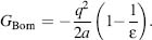
Qualitatively it can be thought of as the distance from the atom to the molecular surface. Accurate estimation of the effective Born radii is critical for the GB model and has undergone much advancement in recent years. Thus, recent methodological advances have pushed the level of accuracy and complexity of continuum electrostatics-based solvation theories, providing the means to efficiently and accurately expand motion simulation to longer timescales.
Minimization Schemes
Energy minimization—moving the system to a local minimum on the energy landscape is an essential step for analyzing the macromolecular structure as well as for preparing the coordinates for a time-dependent simulation. Any given structure of a macromolecule is likely to contain errors often referred to as energetic “hot spots.” Even in high-resolution structures, steric clashes as well as side-chain flips of residues such as Asn, Gln, and His are not uncommon (Chapters 14-15). Other common inaccuracies include salt-bridges that are not optimized, poor packing between atoms, and missing solvent molecules within internal cavities. Moreover, macromolecular simulation is conducted using FFs that are intrinsically inaccurate. Consequently, even a structure of the highest possible resolution will have local hot spots that can be relaxed by a simple minimization. Complimentary, a structure minimized by one FF will have to be minimized again if moving to a different FF.
The definition of a “local” minimum depends on the energy minimization scheme. While there may be deep energy wells in the energy landscape that are masked by energy barriers, the aim of most energy minimization schemes is to overcome (or “polish”) the energy surface roughness for the identification of a more significant local energy minima. FFs are built from components that are deliberately easily derivable. A one-dimensional minimization to the X0 minimum can be written as a Taylor expansion:
(37.9)
with F’ and F being the first and second derivatives of the energy function described by the FF. Moving to a multidimensional function requires the replacement of the derivatives by the gradient and the minimum point by a vector. The accuracy of the minimization depends on the number of computed components within the Taylor expansion. Minimization algorithms that do not include derivation, for example, grid search, are termed zero-order methods. A first derivative of the function, termed first-order methods, utilizes the gradient of the potential energy surface. The most popular of these are the steepest descent minimization (SDM) and the conjugated gradient minimization (CGM) methods. Second derivative methods (order two algorithms), for example, the Adapted Basis Newton-Raphson (ABNR), include the use of information about the curvature.
SDM moves the coordinate system in a direction that corresponds to the change in the gradient of forces exerted on the system by the FF energy function. The first step of this iterative process is of a predetermined arbitrary size. If the SDM step provides a lower energy, it is assumed that the structure is moving to a lower place on the energy surface so the next step size is increased, for example, by 20%. On the contrary, if the resulting energy is higher it is assumed that a local energy barrier was encountered so in order to confirm that the system is not moving out of the local energy well, the next step size is decreased, for example, by half. SDM is efficient in relaxing local barriers and in finding the local minima basins, yet it is also likely to fluctuate out of “shallow” basins.
CGM is another first-order minimizer that is computationally slightly less efficient than SDM. The advantage of CGM is that the minimization solution for the system is closer to the local minima compared to SDM with the use of “memory” for previously calculated gradients. After the first step, the direction of the minimization is determined as a weighted average of squares of the current gradient and the direction taken in the previous step. CGM converges much better than SDM and partially overcomes the problem of fluctuating around the minima. As CGM accumulates numerical errors it is usually restarted every predetermined number of steps.
Order two minimization algorithms make use of the curvature (Hessian) and not only the slope (gradient) of the FF function. The Newton-Raphson algorithm assumes that, near the minimum, the energy can be approximated to be a quadratic function. For the one-dimensional function the minimum can be approximated as X — F’(X0)/F’’(X0). For the multidimensional minimization, the first derivative divided by the second derivative is the gradient divided by the Hessian. Beyond the nonquadratic form of the energy function, calculation of the Hessian repeatedly is inefficient. Consequently, the ABNR (Brooks et al., 1983) is used. ABNR utilizes the curvature information only for the few atoms that contributed the most to the previous move, thus reducing the computation to a small subspace and achieving efficiency that is not far from the CGM algorithm.
An optimized minimization protocol usually takes advantage of these three minimization schemes by applying them sequentially. The crude SDM brings the system quickly to a lower region on the energy landscape where it is replaced by the more accurate CGM and finally refined by ABNR. The termination criterion of each step is often defined in terms of reaching to a gradient root-mean-square-deviation (GRMSD) threshold. If the threshold is not reached, the minimization scheme is replaced after a predetermined number of steps.
Molecular Dynamics—Moving the System
In classical MD, the forces are formulated according to the classical Newtonian equations of motion. A standard Taylor expansion provides the formalism for the move of position x(t)to a position after a short and finite time interval Δt:
(37.10)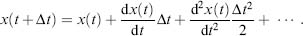
The Taylor series is composed of the position, the velocity and the acceleration of the system. In order to comply with Newton’s third law--conservation of total energy and momentum, computation of these terms are not sufficient. Finite-difference integration algorithms are utilized in which the integration is divided into small steps of future and past time. The Verlet algorithm (Verlet, 1967) uses the time of x(t — Δt):
(37.11)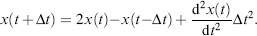
The integration requires only a single force evaluation per iteration. Further, this formalism guarantees time reversibility, as required for ergodic behavior. Yet, it is not “self-starting,” requiring a lower order Taylor expansion to initiate propagation. Moreover, it must be modified to include velocity-dependent forces or temperature scaling. The computationally slightly more expensive leapfrog algorithm (Hockney, 1970) reduces numerical errors and improves velocity evaluation as it uses “half-time steps and gradient information:
(37.12)
(37.13)
To further increase accuracy and numerical stability, the slightly more computationally intensive Verlet velocity algorithm is utilized. This Verlet-type half-time step (like leapfrog) algorithm synchronizes the calculation of positions, velocities and accelerations without sacrificing precision.
The use of dynamic integrators may bias the system considerably. To reproduce an experimental condition, all computed coordinates should belong to a single macroscopic or thermodynamic state. Namely, the characterized ensemble should be constrained to fixed thermodynamic properties. Properties that can be fixed include the number of atoms (N), volume (V), temperature (T), pressure (P), enthalpy (H), chemical potential (μ), and energy (E). Correspondingly, the ensembles include the popular NVT canonical ensemble, the NPH isobaric-isoenthalpic ensemble, the NPT isobaric-isothermal ensemble, the μVT grand canonical ensemble, and the NVE microcanonical ensemble in which the energy conservation implies a closed system. While the Newtonian equations of motion imply energy conservation, NVE does not represent common experimental conditions and may result in an energy drift. To keep these constant conditions, the system must be monitored and corrected accordingly. For example, velocities can be rescaled to maintain constant temperature or volume can be adjusted to maintain a constant pressure. Alternatively, the Andersen (Andersen, 1980) or the Berendsen (Berendsen et al., 1984) thermostat couples an external bath of constant temperature to provide an NVT ensemble. These thermostats are often applied via a velocity Verlet algorithm. The Langevin thermostat (Grest and Kremer, 1986) applies stochastic forces and a dampening friction coefficient. The so-called “hot solvent-cold solute” is a known challenge that arises from the higher sensitivity of the solvent to simulation noise. This may also cause a differential effect on different parts of the macromolecule, for example, flexible tails. Consequently, care should be given to the level of coupling to the external bath and the Langevin thermostat may be preferred for inhomogeneous systems (Mor, Ziv, and Levy, 2008). Similarly, the constant pressure method of Andersen (1980) was developed by Nose and Klein for noncubic cells. It includes an additional degree of freedom—a piston corresponding to the volume, which adjusts itself to equalize the internal and applied pressures maintaining a NPH ensemble (Nose and Klein, 1983). Constant pressure MD algorithms were developed by maintaining volume and temperature thus providing an NPT ensemble (Martyna, Tobias, and Klein, 1994). Later, Feller et al. replaced the deterministic equations of motion for the piston degree of freedom by a Langevin equation thus introducing the popular Langevin piston for maintaining an NPT ensemble (Feller et al., 1995).
The selection of the minimal time step (Δt) for which the dynamics are calculated affect the computational cost directly. Moving to a longer time step without affecting accuracy can be applied by freezing the fastest modes of vibration, namely, constraining the bonds involving hydrogen atoms to fixed lengths. The SHAKE (Vangunsteren and Berendsen, 1977), RATTLE (Andersen, 1983) and LINCS (Hess et al., 1997) algorithms all aim at this higher efficiency. For example, SHAKE applies a constrained Verlet method to the velocities. LINCS resets the constraints directly (rather than their velocity derivative) thus avoiding the accumulating drifts. The constraints can be solved via matrix inversion (MSHAKE) to receive higher accuracy with an additional computational cost. Other variations include the introduction of quaternion dynamics for rigid fragments (QSHAKE). Notably, the use of such efficiency adding algorithms should be used with care. For example, these algorithms will alter the evaluation of temperature that is directly computed from the atomic velocities of all atoms in the system.
The use of multiple time-step dynamics can be expanded beyond the fast fluctuations of the hydrogen atoms and easily integrated into the dynamic integrator. As certain interactions evolve more rapidly than others, forces within the system can be classified according to the variation of the force with time. Taking advantage of the additivity of the FF, each force constituent is integrated in a different time step. The reversible reference system propagator (r-RESPA) allows such extended time steps to be utilized (Tuckerman, Berne, and Martyna, 1992). Similarly, the r-RESPA scheme may be utilized to couple the system to the fast multiple method (Zhou and Berne, 1995). Typically, the bonded interactions, the Lennard-Jones interactions and the real-space part of the electrostatic interactions are computed every 2 fs, while the Fourier-space electrostatics is computed every 6 fs.
Another approach to overcome the limitations of a slowly evolving single trajectory is to enhance the dynamics of part of the system or the entire system. Approaches include applying an elevated temperature, using multiple copies of regions of the system or adding a biasing force to direct the dynamic propagation toward the investigated goal. The first group of methods includes an unbiased enhanced sampling of the system. In the locally enhanced sampling, introduced by Elber and coworkers (Czerminski and Elber, 1991), a fragment of the system is duplicated into noninteracting copies. The strength of each copy to the remainder of the system is downscaled according to the overall number of copies. While a single to multicopy perturbation is required prior to the simulation and then the reversible at the end of the simulation, this method demonstrates quick convergence in cases involving an unknown phase space that is confined to a small region of the system. More generally, the entire system can be represented by multiple copies—an approach well fit to distributed computing such as the folding@home project (Snow et al., 2002). Applying multiple 5-20 ns MD simulations, this approach provided a motion simulation of a large ensemble of a mini-protein providing dynamic description that was well validated via experimental temperature-jump measurements. A multiple copy approach can also be applied as a mean to rapidly overcome local energy barriers. The parallel tempering method and the replica exchange MD (denoted REMD; Sugita and Okamoto, 1999) utilizes noninteracting replicas at different temperatures. Using a Monte Carlo transition probability the replicas swap by reassigning velocities. The method is well fit for small molecules but is considered to be rather slow for full conformational sampling of large macromolecules. REMD was recently applied as a tool of increased sampling of conformational space, for example, for refining homology models (Zhu et al., 2008) and to explore the zipping and assembly of a protein folding model (Ozkan et al., 2007). In essence, these steered MD methods are the theoretical analogy to experimental single molecule experiments such as force microscopy or optical tweezers (Sotomayor and Schulten, 2007). However, unlike the experimental procedure, the theoretical one provides a full movie of the macromolecular dynamics. Steered MD is well fit to explore significant structural changes such as ligand binding and unfolding providing insight into elasticity and local stabilizing features within the macromolecule.
Taken together, classical MD methods provide a valuable tool to explore macromolec-ular motion in timescales approaching several microseconds. In order to achieve such long timescales without compromising on simulation accuracy, software that can be run in parallel is required. Examples of such software packages include the NAMD (Nelson et al., 1996) freeware as well as IBM’s Blue Matter (Germain, 2005) (customized for the Blue Gene computer) and Desmond (Bowers et al., 2006) of DE Shaw Research. Interestingly, NAMD also runs highly efficiently on the Blue Gene computer (Kumar et al., 2008). Examples of power computing conducted with these software packages include a 15 ns NAMD-based simulation of the large aquaporin tetramer embedded in a solvated membrane (Tornroth-Horsefield et al., 2006), a 2.6 Lis Blue Matter-based simulation of the role of direct interactions in the modulation of rhodopsin by co-3 polyunsaturated lipids (Grossfield, Feller, and Pitman, 2006), and a 3 Lis Desmond-based simulation of the NhaA Na+/H+ antiporter (Arkin et al., 2007). These membrane protein simulations exemplify the new biological insight now available with classical MD simulations coupled and optimized to run on supercomputers. Hence, coarse-grained and full atomistic membrane protein MD forms a major target for the growing and increasingly important field of protein motion simulation (Saiz and Klein, 2002; Roux and Schulten, 2004; Gumbart et al., 2005; Brannigan, Lin, and Brown, 2006; Feller, 2007; Kandt, Ash, and Tielman, 2007; Lindahl and Sansom, 2008).
Langevin and Brownian Dynamics
Newton’s equation of motion (second law) states that the force is the mass multiplied by the acceleration (F = ma). In some cases, the Newtonian equation may be replaced by a stochastic equation of dynamics for the solute-solvent interactions, thus increasing the conformational sampling. The Langevin equation adds a drag force representing friction due to the solvent and a random force that represents stochastic collisions between the solvent and the solute. Schematically, for the one-dimensional space, the Langevin equation is
(37.14)
where ζ is the friction coefficient and R(x) the random force. A correction term, termed “mean force” may be added to the equation to represent an average effect of degrees of freedom not explicitly treated by the simulation.
In cases of substantial displacement of the solute, the internal forces may be sufficiently low, relatively, so the dynamics represent a random walk within the viscous environment. Brownian dynamics, the diffusional analog of the MD method necessitates that the friction coefficient within the Langevin equation is sufficiently large resulting in a random walk diffusional trajectory. Thus, Brownian dynamics are fit for diffusion-controlled reactions. Protein-protein interactions as well as ligand biding and channeling are just some of these applications (Gabdoulline and Wade, 2002). Improving sampling for slow association events may be applied via steered Brownian dynamics (Zou and Skeel, 2003).
QM-MM METHODS
In 1976 Warshel and Levitt (1976) studied the lysozyme active site via QM-MM, establishing a field that has become widespread in the study of biomacromolecules. The simplified model for protein folding introduced by them in 1975 (Levitt and War-shel, 1975) is now emerging as one of the methods of choice for studying protein folding. While QM calculations are computationally far more intensive compared to the reduced MM representation, the large increase in accuracy often requires their utilization (Senn and Thiel, 2007; Dal Peraro et al., 2007a; Friesner and Guallar, 2005). This is especially the case for the most interesting part of the protein--the active site or the ligand/cofactor binding region. Understanding time-dependent changes within such regions in the best possible accuracy is important for understanding the key function of the macromolecule. Furthermore, some of the intrinsic characteristics of such regions are quantum effects that form intrinsic limitations for classical dynamics applications. These include (a) parameterization of highly conjugated systems or tunneling of electrons/ protons, (b) bond rearrangement chemistry and other chemical processes where the change in the electronic structure, for example, through excitation is pivotal, and (c) parameterization of atom groups other than the common amino acids and nucleic acids for which most FFs have been tailored for. As such, the reactive region subjected to QM computation should be of sufficient size to encompass any important electronic structure effects.
In QM-MM simulations, a small area of interest is treated by QM electronic structure theory, the majority of the protein and aqueous solvent is represented by a FF, and the boundary between the two regions is uniquely treated to ensure that large errors are not made in coupling the two regions. The exact form of the coupling terms and the details of the boundary region define the specific QM-MM scheme.
The QM-MM scheme can be applied with most types of QM methods. In the scope of this introductory chapter the QM aspect can be only briefly introduced. In the Schrödinger equation, an electron is described as a unique wave function describing the quantum state of the electron. The computation of many-electron wavefunctions is complex for large molecules and so approximate schemes have been developed that have been parameterized to overcome many of their intrinsic shortcomings. One of the common approaches nowadays is to work with the electron density as the basic quantity, which is referred to as density functional theory (DFT). It turns out that DFT is computationally a simpler quantity to deal with. Yet, the main limitation of DFT is the inherent inability to describe the London dispersion forces underlying van der Waals interactions. However, empirical approaches are currently being developed to overcome this deficiency.
First principles QM alone can only yield the molecular structure at the local minima (or saddle point important for reaction pathway). Consequently, entropic temperature effects cannot be readily incorporated. To enable the calculation of free energy effects, the QM has to be incorporated within an MD scheme that includes temperature effects and thus can benefit from established statistical mechanics methods such as steered dynamics or umbrella sampling. DFT was first applied within MD framework by Car and Parrinello (1985), forming the commonly utilized CPMD simulation. In CPMD, the electronic degrees of freedom are treated as dynamical variables and the resulting fictitious electron dynamics are coupled to the classical dynamics of the nuclei. At present, up to hundreds of atoms may be simulated to times in the order of hundreds of picoseconds.
CPMD can be coupled to classical MM MD yielding a dynamical QM-MM scheme. The key in combining the combined electronic structure and dynamics scheme within a classical protein FF-based dynamics simulation scheme is the specification of the coupling interface between the quantum QM and classical MM regions. If the two regions are not covalently linked, the challenge is reduced to the parameterization of nonbonded interactions between the MM and QM atoms. However, commonly the regions are covalently bonded requiring more special treatment. The simplest way to treat the interface is to cap the QM-computed moiety by hydrogens or pseudoatoms and treat the two entities distinctly, possibly adding correction terms. An alternative method is the use of a frozen orbital on the bond(s) connecting the regions. Here, the electronic structure equations are solved for the QM region incorporating the electron density of the frozen orbital as well as the charge distribution originating from the MM region.
From the first study on the stabilization of the carbonium ion with the lysozyme enzyme, current QM-MM methods aid in understanding enzymes. The approach is especially applicable for nonprotein moieties integral to protein complexes such as met als. For example, Dal Peraro et al. applied a QM-MM approach to capture the mean polarization and charge transfer contributions to the interatomic forces within protein met al sites, resulting in better MD simulations enabling relaxation of local frustrations in NMR structures (Dal Peraro et al., 2007b). The free energy perturbation method to calculate the free-energy differences along the path is facilitated by the approximation of replacing the QM density by atomic charges fitted to the electrostatic potential. Enzyme reactivity is a prime target of QM-MM simulations. Specifically, it is usually difficult to model bond rearrangements and transition state stabilization via conventional MM dynamics. Similarly, QM-MM dynamics can expand the usage of MM dynamics to the simulation of electronically excited states, for example, chromophore photoactivated isomerization in the photoactive yellow protein (PYP; Groenhof et al., 2004) or in rhodopsin (Gascon, Sproviero, and Batista, 2006). Hence, with the rapid growth in computer power, the usage of QM-MM dynamics is expected to grow and provide high-resolution understanding of structure-function relationships within biomacromolecules.
CONCLUSION
The field of motion simulation has matured into a central component of understanding macromolecule dynamics. Recently, the field has benefited from evolving methodological advances along with continually increasing computational power and the concomitant increase in experimental structural and biophysical data. The combination of atomistic simulations based on detailed intermolecular FFs with longer timescale coarse-grained simulations bridges the gap in our understanding of macromolecular motion. No less important, development in experimental methods and the increasing synergy between experiments and simulation assist in validating models of macromolecules and self-assembled structures. Long MD simulations imitating experimental conditions provide a detailed dynamic understanding of experimental results, for example, simulating the folding of a mutated lyzosyme (Zhou et al., 2007; Figure 37.4). Consequently, the role of MD simulations in understanding macromolecular dynamics is expected to increase; expanding in accuracy of results, length of time studied and size of systems analyzed.
Although addressed throughout the chapter, we wish to emphasize once again that the appropriate choice for a simulation study of motion depends on the desired analysis, required resolution of dynamic information, and consideration of the system to be simulated. The main tradeoff involves the desired resolution of motion to be modeled and the computational demands. In addition, the dynamical simulation toolbox should be viewed as another component in the understanding of motion. The emerging integration of simulation techniques with established and emerging experimental and bioinformatic methods provides a way to understand the dynamics in a validated manner. As the data for protein motion accumulates from various experimental resources, this will fuel research focus aimed to understand how functional motion is encoded at the sequence level (Gu et al., 2006). Hence, the field of protein motion simulation is expected to expand in depth, breadth and importance to the biological community.
See notes on relevant books at the references reading section of Chapter 8.
ACKNOWLEDGMENTS
Thanks to Christopher M. MacDermaid for critical reading of the manuscript. IS thanks the European Molecular Biology Organization (EMBO) and the Human Frontier Science Program Organization (HFSPO) for support. MLK thanks the NIH for support.