5
MACROMOLECULAR STRUCTURE DETERMINATION BY NMR SPECTROSCOPY
Bioinformatics plays an important role in biomolecular structure determination by NMR spectroscopy. Increasingly, structural biology is being driven by information gained from gene sequencing and hypotheses derived from bioinformatics approaches. This is particularly so for structural proteomics efforts. A major rationale for structural proteomics is that a more complete mapping of peptide sequence space onto conformational space will lead to efficiencies in determining structure-function relationships (Burley, 2000; Heinemann, 2000; Terwilliger, 2000; Yokoyama, 2000). Longer range scientific goals are the prediction of structure and function from sequence and simulations of the functions of a living cell. Structural proteomics is part of a wider functional genomics effort, which promises to assign functions to proteins within complex biological pathways and to enlarge the understanding and appreciation of complex biological phenomena (Thornton et al., 2000). Because of its potential to greatly broaden the targets for new pharmaceuticals, structural proteomics is expected to join combinatorial chemistry and screening as an integral approach to modern drug discovery (Dry, McCarthy, and Harris, 2000). It is clear that much larger databases of structures, dynamic properties of biomolecules, biochemical mechanisms, and biological functions are needed to approach these goals. Because of its ability to provide atomic-resolution structural and chemical information about proteins, NMR spectroscopy is positioned to play an important role in this endeavor. Already, NMR spectroscopy contributes about 15% of the protein structures deposited at the Protein Data Bank (PDB). In addition, NMR spectroscopy is used routinely in high-throughput screens to determine protein-ligand interactions (Mercier et al., 2006; Hajduk and Greer, 2007). NMR also is a key tool in mechanistic enzymology and in studies of protein folding and stability. As discussed here, advances in key technologies promise rapid increases in the efficiency and scope of NMR applications to structural and functional genomics. Bioinformatics figures prominently in these advances.
This Chapter discusses the current status and prospects of macromolecular structure determination by solution state NMR spectroscopy. Although the focus is on proteins, the approaches can be generalized to other classes of biological macromolecules. Solid-state NMR spectroscopy shows great promise for structural studies of proteins that may not be amenable to investigation in solution, such as membrane proteins, and for functional investigations of protein in the solid state. Solid-state NMR strategies for biomolecular sample preparation, data collection, and analysis are developing rapidly and are expected to assume prominence in the next few years. Further discussion of this highly specialized field is beyond the scope of this chapter, and interested readers are directed to recent reviews (McDermott, 2004; Baldus, 2006; Hong, 2006).
This chapter starts with an overview of the physical basis for NMR spectroscopy and a discussion of NMR experiments and instrumentation. Then, the basic approaches used in determining structures and dynamic properties of proteins are presented. Sample requirements and sample preparation, including labeling methods, are discussed. Next a protocol for NMR structure determination covering all steps from protein characterization to data deposition is detailed. This is followed by a section on evolving bioinformatics technology for achieving a more automated, probabilistic approach to protein NMR structure determination. The final section summarizes various bioinformatics resources that are available to support biomolecular NMR spectroscopy.
INTRODUCTION TO PROTEIN STRUCTURE DETERMINATION BY NMR
Comparison of NMR Spectroscopy and X-ray Crystallography
Current methods for high-throughput protein structure determination are single-crystal diffraction and solution-state NMR spectroscopy. The two methods have complementary features, as X-ray crystallography represents a mature and rapid approach for proteins that form suitable crystals while NMR has advantages for structural studies of small proteins that are partially disordered, exist in multiple stable conformations in solution, show weak interactions with important cofactors or ligands, or do not crystallize readily. NMR spectroscopy is an incremental method that can rapidly provide useful information concerning overall protein folding, local dynamics, existence of multiple folded conformations, or protein-ligand or protein-protein interactions in advance of a three-dimensional structure. This information can be useful in designing strategies for 3D structure determinations by either NMR or X-ray crystallography. Several ongoing structural proteomics pilot projects are employing a combination of X-ray crystallography and NMR spectroscopy.
Physical Basis for Biomolecular NMR Spectroscopy
As summarized schematically in Figure 5.1, NMR spectroscopy investigates transitions between spin states of magnetically active nuclei in a magnetic field. The most important magnetically active nuclei for proteins are the proton (1H), carbon-13 (13C), nitrogen-15 (15N), and phosphorus-31 (31P). Each of these stable (nonradioactive) isotopes has a nuclear spin of one half and, as a consequence, two spin states: one at lower energy, with the magnetic spin paired with the external field, and one at higher energy, with the magnetic spin opposing the external field. The magnetic moment of each nucleus precesses about the external magnetic field and is influenced by other fields. Influences on a given spin are generated by neighboring spins in the molecule, giving rise to intrinsic NMR parameters, or by radiofrequency pulses and/or pulsedfield gradients as programmedby theNMRspectroscopist. In an NMR experiment, a time sequence of radiofrequency pulses and pulsed field gradients are applied to the spins present in the molecule studied. The excited spins are allowed to interact with one another and with the externalmagnetic field. Then, the state of the system is read out by detection of the current induced by the nuclear spins of the sample in the receiver coil of the NMR spectrometer. The physical basis for NMR is well understood, and the spectroscopic consequences of a given pulse sequence applied to a particular molecule can be simulated to a good level of precision (Cavanagh et al., 2006; Ernst, Bodenhausen, and Wokaun, 1987).
Figure 5.1. Schematic illustrating several basic principles of biomolecular NMR spectroscopy. (Clockwise from upper left) The NMR sample solution is placed in an NMR tube, which is then inserted into the static magnetic field of the NMR spectrometer. NMR-active nuclei (e.g., 1H, 13C,and 15N) within the sample precess (like a spinning gyroscope) with their net magnetization aligned with the direction of the magnetic field; the precession frequency is governed by the type of nucleus but is modulated by the chemical environment of the atom in the macromolecule. Application of a radiofrequency pulse excites the nucleus by flipping its spin to the excited energy level opposing the external magnetic field. A “90 pulse” flips the rotating magnetization into the plane perpendicular to the axis of the magnetic field (the “x-y plane”), and the rotating magnetization induces an oscillating current (the “free induction decay”) into the coil that detects the signal. Fourier transformation of the time-domain signal (free induction decay) converts it to a frequency-domain signal (the “NMR peak”). More complicated pulse sequences are used in experiments that create two- or three-dimensional NMR spectra; the type of 3D spectrum illustrated is the result of a “triple resonance” experiment in which the three orthogonal frequency axes display the peak positions of combinations of 1H, 13C, and 15N nuclei that are related by spectral connectivities created by the pulse sequence.

NMR Experiments
The NMR spectrometer can be programmed to operate on sets of nuclei of single or multiple atom types and to accommodate particular spectral features (chemical shift range, spin-spin coupling range, etc.). NMR spectroscopy is unique in that the Hamiltonian ofthe system under study can be manipulated easily by the application of radiofrequency pulses and/or pulsed field gradients. The versatility in creating sequences of complex “spin gymnastics” makes possible a myriad of NMR experiments by which particular parameters can be investigated. A huge variety of NMR experiments are at one’s disposal when collecting data for a structure determination or functional investigation. The NMR field is still young and dynamic, and these experiments continue to evolve; thus the optimal set of experiments for a structure determination or structure-function study is a matter of exploration and individual taste. The approaches described here are ones that we have found to be effective.
Structure from NMR
The classical approach to structure determination is to first use multidimensional and multinuclear NMR methods to determine “sequence-specific assignments,” that is, resolve signals from the 1H, 15N, and 13C nuclei of a protein and to assign them to specific nuclei in the covalent structure of the molecule. The assigned chemical shifts (cs) themselves provide reliable information about the secondary structure of the protein (Wishart, Sykes, and Richards, 1992; Wishart and Sykes, 1994a; Wishart and Case, 2001; Eghbalniaet al., 2005c), and the oxidation states of cysteine residues (Sharma and Rajarathnam, 2000), and can be used to test or validate structural models. Additional structural restraints are obtained from an interpretation of data from one or more different classes of NMR experiments: nuclear overhauser effect (NOE) spectra, which provide 1H — 1H distance constraints; empirical torsion angle constraints based on chemical shifts (Cornilescu, Delaglio, and Bax, 1999); and (3) residual dipolar couplings from partially oriented proteins (Bax, Kontaxis, and Tjandra, 2001; Lipsitz and Tjandra, 2004; Prestegard, Bougault, and Kishore, 2004; Bax and Grishaev, 2005), which provide spatial constraints (with respect to the orientation axes) for pairs of coupled nuclei. Additional hydrogen bond constraints are determined from hydrogen exchange experiments, chemical shifts, and/or trans-hydrogen bond couplings (Cordier and Grzesiek, 1999; Cordier et al., 1999).
Molecular Size Limitations
Protein NMR methods have advanced to the point where small to medium sized protein domain structures can be determined in a routine manner. Key milestones in the development of this technique include NOE-based resonance assignment and structure refinement (Wuthrich, 1986), efficient stable isotope labeling methods (Markley and Kainosho, 1993), detection of multinuclear correlations (Westler, Ortiz-Polo, and Markley, 1984; Ortiz-Polo et al., 1986; Oh et al., 1988; Westler et al., 1988a, 1988b; Oh, Westler, and Markley, 1989) coupled with indirect detection and multinuclear NMR spectroscopy (Kay, Marion, and Bax, 1989; Kay et al., 1990). More recent advances have included the use of pulsed field gradients for coherence selection and line-narrowing by transverse relaxation-optimized spectroscopy (TROSY) (Czisch and Boelens, 1998; Pervushin et al., 1998; Salzmann et al., 1998; Zhu, Kong, and Sze, 1999; Zhu et al., 1999; Fernandez and Wider, 2003; Hu, Eletsky, andPervushin 2003). Theimprovements incommerciallyavailableNMRhardware and remarkable advances in desktop computing capabilities have also been important.
Protein domains of up to roughly 25 kDa generally are amenable to high-throughput NMR structure determination, provided that soluble, stable, U — 13C- and U — 15N-labeled samples can be obtained. This isotope enrichment enables the use of sensitive multinuclear correlation experiments for the task of matching all chemical shifts in the protein with specific amino acid residues and atoms. Once all 1H, 15N, and 13C resonances have been assigned, the correlations observed in nuclear Overhauser enhancement experiments can be interpreted in terms of short (< 5Å) inter-proton distances. NMR structures are obtained from constrained molecular dynamics calculations, with these NOE-derived 1H--1H distances as the primary experimental constraints. As a consequence of chemical shift degeneracy, many NOE correlations may have multiple assignment possibilities, and the results of preliminary structure calculations are used to eliminate unlikely candidates on the basis of inter-proton distances. Refinement continues in an iterative manner until a self-consistent set of experimental constraints produces an ensemble of structures that also satisfies standard covalent geometry and steric overlap considerations. Recent advances in software have automated many of the steps in structure determination (Lopez-Mendez and Guntert, 2006). Structures are validated and reported in the Protein Data Bank in a manner analogous to those obtained from X-ray crystallographic methods (see Chapters 14 and 15).
Stable Isotope Labeling
Structures of smaller proteins can be determined with samples at natural abundance. If the protein is reasonably soluble (≥ 1 mM), and particularly if a high-sensitivity cryogenic probe is available, it is possible to obtain 1H-13C and 1H-15N correlations at natural abundance. This additional information can be useful for signal assignments and to provide additional chemical shifts for secondary structure analysis. These structures are generally of lower quality than those determined from labeled proteins because of the greater difficulty in obtaining complete assignments. High-throughput strategies for protein structure determination generally are designed for proteins ’double-labeled’ with 13C and 15N (Mr >~25,000 Da) or “triple-labeled” with 13C, 15N, and 2H(Mr <~25,000 Da). NMR spectra of larger molecules are characterized by increasingly rapid decay of the signal to be detected leading to increased line widths and lowered sensitivity (signal-to-noise ratio) and by greater overlap and signal degeneracy. Even with triple-labeled proteins, these problems make it increasingly difficult to solve NMR structures of proteins larger than 40 kDa with current methodology. Using higher magnetic fields and TROSY methodology suggests that these limitations can be overcome to some extent. Kay and coworkers have developed a labeling strategy for large molecules by 15N, 13C, and 2H labeling while the methyl groups of isoleucine, leucine, and valine are protonated (Gardner and Kay, 1998; Tugarinov, Kanelis, and Kay, 2006).
Selective labeling approaches make it possible to obtain information about selected regions of proteins as large as 150 kDa. These methods include labeling by single residue type (Markley and Kainosho, 1993) and segmental labeling by peptide semisynthesis, including intein technology (Yamazaki et al., 1998; Xu et al., 1999). In the designer labeling scheme, known as stereo-array isotope labeling (SAIL) (Kainosho et al., 2006), a complete stereospecific and regiospecific pattern of stable isotopes is incorporated into the protein using cell-free protein synthesis. SAIL, by significantly reducing the proton density and thus reducing the resonance overlap and line width, has great potential in extending the molecular weight range for structure determination by NMR.
Data Collection and Instrumentation
Even with protein sample concentrations in the millimolar range (> 10 mg/mL), coaddition of 8 or 16 transients may be required at each time point in some two- or three-dimensional experiments to achieve sufficient signal-to-noise (s/n). Cryogenic probe technology can reduce the data acquisition period by up to a factor of 10. This results from the three- to fourfold enhancement in sensitivity achieved by cooling the probe and preamplifier circuitry to very low temperatures (Styles et al., 1984). Because of the square-root relationship between time and sensitivity in signal averaging, an inherent sensitivity improvement of threefold is equivalent to a ninefold increase in signal averaging. In practical terms, the s/n of an experiment acquired with one or two transients at each time increment on a cryogenic probe should be equivalent (if not superior) to one acquired with 16 transients using a conventional (noncooled) probe. For this example, the cryogenic probe results in an eightfold reduction in experiment time with no negative consequences. This is especially important for NOE experiments. There are some caveats associated with the use of cryogenic probes. First, the three- to fourfold sensitivity increases generally are realized only for simple 1D experiments in nonionic solutions. The RF field inhomogeneity of the 13C and 15N coils decreases the efficiency of the probes in multipulse triple-resonance experiments. Practically, for a protein solution at low ionic strength, the sensitivity increase is closer to twofold. However, this increase yields either a fourfold saving in time or, more importantly for systems of poor solubility, the ability to lower the sample concentration by a factor of two. The most severe limitation of the cryogenic probe is that they lose their sensitivity advantage in solutions having high ionic strength. Recent studies have shown that by changing the shape of the sample tube to limit the penetration of the electric field into the salty solution, the sensitivity can be recovered even in solutions of high ionic strength (de Swiet, 2005).
Approaches for decreasing the overall experimental time by collecting sparse data sets have been developed, such as HIFI (Eghbalnia et al., 2005a), GFT (Kim and Szyperski, 2003), and reconstruction of 3D from 2D planes (Kupce and Freeman, 2003). These methods decrease the collection time simply by collecting projected 2D planes out of a 3D spectrum and can reduce the data collection time by nearly an order of magnitude. The ultimate limit for rapid data collection is the longitudinal relaxation rate of the nucleus to be detected. Data collection schemes, such as “SOFAST,” that use optimal recycle rates have produced 2D spectra in less than 1 min (Schanda and Brutscher, 2005), and these strategies have been developed into a suite of pulse sequences for triple-resonance data collection (Lescop, Schanda, and Brutscher, 2007).
Protein Dynamics from NMR
NMR signals report on the chemical properties of nuclei including their relative motions with respect to the magnet and molecular frames. Consequently, NMR spectroscopy is uniquely suited for investigations of the kinetics and thermodynamics of molecular motions, segmental motions, dynamic conformational equilibria, and ligand binding equilibria— as reviewed in greater detail elsewhere (Palmer III, Kroenke, and Loria, 2001; Wand, 2001; Kern and Zuiderweg, 2003; Mittermaier and Kay, 2006). Whereas regions of proteins that are statically or dynamically disordered may fail to produce resolvable electron density, NMR signals from such regions generally are observed and can be investigated (Dyson and Wright, 2005).
Dynamic processes observable by NMR spectroscopy cover a vast timescale: from picoseconds to seconds, days, and even months. Nuclear spin relaxation rates are sensitive to protein motions ranging from picosecond to milliseconds. Overall molecular tumbling on the nanosecond timescale is the dominant factor in relaxation of most nuclei in folded proteins. Internal protein motions on the picosecond timescale cause a slight averaging of the dipolar interactions that in turn reduces the overall spectral density. These variations can be measured for the backbone of each residue in a protein by determining the time constants for 15N longitudinal (T1) and transverse (T2) relaxation rates as well as the 1H(15N) heteronuclear NOE (Palmer, 1997). Analogous measurements of 2H or 13C relaxation parameters can yield information on side chain dynamics (Igumenova, Frederick, and Wand, 2006).
The motional effect on relaxation rates can be expressed as an order parameter (S2) in a model-free formalism as originally expounded by Lipari and Szabo (1982a, 1982b). Order parameters range from 0 to 1, with smaller values reflecting increased internal motion. Often the simple single exponential model is insufficient to fit the relaxation data, and additional exponentials describing other rapid motions must be added to extend the basic model-free approach (Clore et al., 1990; Mandel, Akke, and Palmer III, 1995). However, it should be noted that as parameters are added to the analysis, the available experimental data points may not suffice to constrain the system to a unique neighborhood of solutions (Andrec, Montelione, and Levy, 2000). Outliers in the transverse relaxation rate often arise from motions in the microsecond-to-millisecond time regime that report on chemical or confor-mational exchange phenomena (Volkman et al., 2001). Relaxation dispersion methods detect these slower motions directly (Akke and Palmer, 1996), and exchange rates have been correlated with protein binding and folding (Sugase, Dyson, and Wright, 2007), rate-limiting steps in enzyme catalysis (Eisenmesser et al., 2005), and even conformational dynamics of the 20S proteasome— a 670 kDa complex (Sprangers and Kay, 2007). For conformational dynamics involving millisecond-to-second interconversion between two or more states giving rise to distinct NMR signals, traditional 2D exchange spectroscopy provides another method for quantification of exchange rates, and ultrafast 2D NMR pulse schemes enable real-time monitoring of kinetic processes on the 1-10 s timescale (Schanda, Forge, and Brutscher, 2007).
Dynamics on longer timescales can be interrogated through hydrogen exchange kinetics (Huyghues-Despointes et al., 2001). In this experiment, a protein that has the natural abundance of 1H atoms on the amide groups is dissolved in a solution containing ~100% 2H2O and then quickly transferred to the spectrometer. By observing the loss of amide 1H signals due to exchange with the 2H atoms, the kinetics can be followed. Protons with larger protection factors are interpreted to be in more highly structured regions with more stable hydrogen bonds. Highly labile protons may exchange completely in the interval between the addition of 2H2O and acquisition of the first NMR spectrum. A complementary method (CLEANEX) for rapidly exchanging amides uses solvent saturation transfer to quantify exchange rates (Hwang, van Zijl, and Mori, 1998). In combination, saturation transfer and H/D exchange measurements can monitor local backbone fluctuations from milliseconds to months. This broad repertoire of NMR methods enables quantitative, site-specific measurement of fast motions and slower conformational exchange process associated with catalysis, allostery, folding, and signaling—central features of most biological processes.
PREPARATION OF PROTEIN SAMPLES FOR NMR
Approaches to Protein Production and Labeling
A variety of protein expression systems have been investigated in support of structural proteomics (Yokoyama, 2003). By far the most widely used and most successful platform is heterologous overexpression of proteins in Escherichia coli cells. It is a general experience, however, that a certain percentage of proteins does not express abundantly in soluble form in bacteria. Insolubility arises either from an intrinsic property of the protein (for example, aggregation due to an exposed hydrophobic surface) or because inappropriate folding mechanisms in the expression host permit aggregation of folding intermediates (Henrich, Lubitz, and Plapp, 1982; Goff and Goldberg, 1987; Chrunyk etal., 1993). Expression can be particularly difficult for eukaryotic proteins that consist of multiple domains, that require cofactors or protein partners for proper folding, or that normally undergo extensive post-translational modification. In industry, the next most widely used approach is protein production from insect cells by a baculovirus system. However, this approach is not widely used for NMR spectroscopy, because labeled media for insect cells are highly expensive. Recently, a more economical medium for Sf9 insect cells has been described, which promises to improve the practicality of this approach (Walton et al., 2006). Yeast cells offer another alternative, and approaches for large-scale production of labeled proteins from the yeast Pichia pastoris have been described (Wood and Komives, 1999; Pickford and O’Leary, 2004).
Cell-free biological systems are capable of synthesizing proteins with high speed and accuracy approaching in vivo rates (Kurland, 1982; Pavlov and Ehrenberg, 1996). Commercial implementations of this technology incorporate recent advances as described below (Spirin et al., 1988; Baranov et al., 1989; Endo et al., 1992; Sawasaki et al., 2002a, 2002b). E. coli cell-free systems give high yields (Kigawa et al., 1999), and active extracts are easily prepared (Torizawa et al., 2004; Matsuda et al., 2007). Membrane proteins can be produced in soluble form by incorporating detergents into cell-free systems (Klammt et al., 2004; Klammt et al., 2006; Liguori et al., 2007). Two groups have made extensive use of cell-free (in vitro) protein production for NMR spectroscopy: the RIKEN Structural Genomics Group (Kigawa, Muto, and Yokoyama, 1995) and the Center for Eukaryotic Structural Genomics (Vinarov, Loushin Newman, and Markley, 2006).
In our experience, a combination of protein production in E. coli cells and in a wheat germ cell-free system provides an economical approach for producing eukaryotic proteins for NMR structural analysis. The two methods are complementary in the sense that many proteins that fail to be produced in soluble, folded state from E. coli can be made from the wheat germ cell-free system, whereas, when production is successful from E. coli, the yields can be very high (Tyler et al., 2005a).
Cell-Based Methods
As noted above, protein production in E. coli has an established record of being the most successful approach for providing protein targets for structural proteomics. Suitable expression vectors are readily available, and the method is more economical than production in eukaryotic cells. Furthermore, promising proteins can be subsequently labeled metaboli-cally with heavy atom-labeled amino acids for X-ray or stable isotopes for NMR (Edwards et al., 2000). 13C—, 15N—, and 2H-metabolic labeling for NMR work was pioneered with E. coli expression systems (Markley and Kainosho, 1993). A recent important advance has been the development of self-induction media containing glucose, glycerol, and lactose for protein production from E. coli, which support very high cell densities while removing the need to follow cell growth to initiate induction and associated centrifugation steps. This approach has been fine-tuned recently to improve yields (Blommel et al., 2007). The approach can be used to produce stable isotope labeled samples for NMR spectroscopy (Tyler et al., 2005b), although the costs for isotopes are higher, because 13C -glycerol must be added in addition to13C-glucose and 15N-ammonia. Additional cost saving can be achieved with E. coli production systems through the use of disposable polyethylene terephthalate (PET) bottles as growth vessels, which do not require cleaning or sterilization (Sanville et al., 2003).
Cell-Free Methods
We have published detailed descriptions of the protocols, which have been developed for the production of labeled proteins for NMR spectroscopy from a wheat germ cell-free system (Vinarov et al., 2004; Vinarov and Markley, 2005; Vinarov et al., 2006). Cell-free protein production methods have several advantages: (1) volumes can be kept manageable—in favorable cases, sufficient protein for a structural investigation can be produced from a reaction volume of under 6-12 mL; (2) proteins can be produced which would be toxic to cells; (3) the ratio of desired protein to unwanted protein is low, simplifying purification; (4) in a cell-free system, one has the potential for introducing metal ions, cofactors, or other agents that promote correct folding; (5) enzymes and substrates can be added to promote post-translational modifications; and (6) labeled amino acids can be introduced without scrambling of the label— this enables clean selective labeling and newer labeling strategies, such as stereo-array isotope labeling (Kainosho et al., 2006).
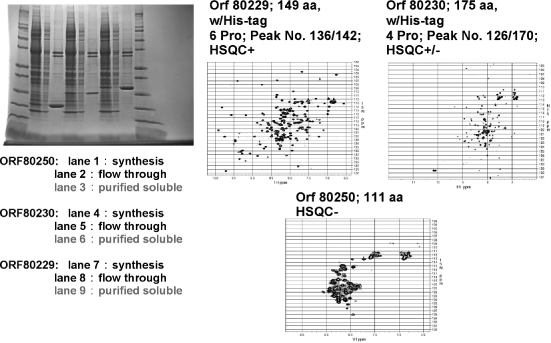
The production of labeled proteins from cell-free systems requires that labeled amino acids be supplied in the reaction mixture. The optimal concentration of each amino acid in the cell-free reaction mixture is about 1 mM. At currently achievable protein yields (0.4-1.1 mg protein/mL of reaction mixture), a reaction volume of 6-12 mL is needed to produce enough protein for an NMR sample. [U-15N]-and [U-15N, U-13C] -amino acids are commercially available at prices that make cell-free protein production of labeled proteins competitive with production from E. coli cells when relative labor costs are taken into account. Figure 5.2 illustrates the automated cell-free production and purification of three protein targets incorporating 15N-amino acids for screening for suitability as structural targets.
Sample Concentration, Volume, and Stability
The higher the protein concentration the faster NMR data can be collected, provided that the protein does not aggregate. Practical lower limit protein concentrations are about 200 μM with ordinary probes and about 60 μM with cryogenic probes. The decreased concentration requirement of the cryogenic probe may make it possible to collect data from proteins that aggregate at higher concentrations. With ordinary NMR tubes, a sample volume of 300-500 μL is required, depending on the length of the detection coil in the probe. Susceptibility-matched cells (Shigemi Inc.) enable the use of smaller volumes: 200 μL in a 5 mm OD tube or 60 μL in a 3 mm OD tube. In cases where the protein is sufficiently soluble (> 1.5 mM), it is possible to use a 1 mm microcoil NMR probe to greatly reduce the amount of protein required (Peti et al., 2005; Aramini et al., 2007).
Figure 5.2. Examples of 15N-labeled His-tagged proteins (two Arabidopsis and one human target) produced by a wheat germ cell-free robotic system (CellFree Sciences DT-II). The robot starts with a DNAplasmid and carries out automated transcription and translation and metal ion affinity protein purification. The SDS gel scans show molecular weight markers on either side, and for each target, the total reaction mixture, column flow-through, and purified soluble fraction seem incomplete. The two bands, at higher molecular weight, correspond to proteins present in the wheat germ extract that bind to the affinity column. They do not show up in the NMR spectra because they are not labeled with 15N. The only manual steps required in preparing the NMR samples were buffer exchange and concentration of the purified protein. The three targets illustrate how 1H-15N HSQC NMR is used to screen targets for their suitability for structure determination. HSQC+ indicates a spectrum with the expected number of well-resolved peaks. HSQC+/- indicates a protein that is partially unstructured and may be salvageable as a structural target by either solvent optimization or by trimming the protein expressed. HSQC indicates a natively unfolded or aggregated protein unsuitable for NMR structure determination (Loushin Newman, Markley, Song, and Vinarov, unpublished results).
The sample must remain stable over the data collection period. If the stability of the sample is a limiting factor, it is possible to use separate samples for different NMR experiments. Ideally, all data sets are collected with the same sample, because slight differences in solution conditions can lead to chemical shift differences that make it difficult to compare results from different experiments. One of the advantages of cryogenic probes and higher fields is that the overall data collection time for each experiment is shortened. This makes it possible to investigate systems that are less stable over time.
PROTOCOL FOR PROTEIN STRUCTURE DETERMINATION BY NMR
As noted above, NMR methodology is evolving rapidly and competing approaches are being explored in various structural proteomics centers. The following sections outline a protocol for semiautomated protein structure determination by NMR spectroscopy. Proteins (≤25 kDa) labeled with 15N emerging from the cell-based or cell-free protein production pipeline are subjected to 1D and 2D NMR screening to determine their folding and aggregation states under a variety of solution conditions (Figure 5.2). Ideally, an NMR spectrometer equipped with a sample preparation robot, sample changer, and cryogenic probe is used for these screens (a 600 MHz system is adequate for this purpose). NMR screens are used to determine aggregation state (through measurement of transverse diffusion by gradient NMR), assess folding state (from analysis of the amide region of 1D 1HNMR spectra and the pattern of1H-15N correlation spectra), monitor ligand binding (by detecting chemical shift perturbations), and survey proteins for the presence of unstructured regions. The results of the NMR screens are used in deciding whether to proceed with NMR structure determination, transfer the protein to the crystallization trials pipeline, or re-engineer the protein to improve its suitability for NMR analysis. This may be accomplished by removing unstructured regions to simplify the 2D and 3D NMR spectra or by isolating individual domains to achieve greater stability or solubility and discourage aggregation (Lytle et al., 2006; Peterson et al., 2007b). Proteins that pass these screens as candidates for NMR structure determination are double-labeled with 15N and 13C as described above.
A 600 MHz NMR spectrometer equipped with a cryogenic probe is well suited to the collection of protein triple-resonance spectra. If available, spectrometers with cryogenic probes operating at or above 750 MHz may be employed in collecting multidimensional NOE and isotope-filtered/selected NOE spectra with enhanced resolution. Measurement of residual dipolar couplings (RDCs) for structure refinement and validation (Tolman et al., 1995; Tjandra and Bax, 1997; Tjandra et al., 1997; Prestegard, 1998; Tian, Valafar, and Prestegard, 2001) requires that samples be partially oriented in the magnetic field. The orientation can be achieved by dissolving the protein in an anisotropic medium, such as phospholipid bicelles (Sanders, Schaff, and Prestegard, 1993; Bax and Tjandra, 1997; Ottiger and Bax, 1999), phage particles (Hansen, Mueller, and Pardi, 1998), or stretched polyacrylamide gels (Chou et al., 2001). Identification of asuitable alignment medium may require additional screening, based on the ranges of pH and temperature that are compatible with the target protein and the degree of association between the protein and medium. In the absence of a robust, “universal” alignment medium, RDC analysis is treated as a supplemental approach to this protocol, and structures are solved using primarily distance constraints derived from NOESY spectra and dihedral angle constraints predicted from chemical shifts. In the absence of RDCs, validation is performed by using a variety of software tools that analyze the coordinates and constraint data.
Standard Data Collection Protocols
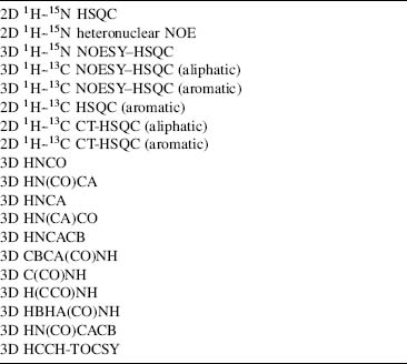
The improved sensitivity from cryogenic probes permits data collection sufficient for a protein structure in 7-10 days, rather than 1 or 2 months. If the protein concentration is sufficiently high that data can be recorded without signal averaging, the total data collection period can be as short as 30 h. The 2D and 3D pulse schemes listed in Table 5.1 have been in routine use in many laboratories for several years.
Updated versions of these pulse sequences that are compatible with cryogenic probes are provided as part of the standard pulse sequence libraries by NMR instrument manufacturers and are available from the NMRFAM web site (<http://www.nmrfam.wisc.edu>) and the BioMagResBank (BMRB) web site (http://www.bmrb.wisc.edu/tools/choose_pulse_info.php). Reduced dimensionality versions of these pulse sequences have also been developed and should yield further reductions in the time required for data acquisition (Montelione et al., 2000; Szyperski et al., 2002; Eghbalnia et al., 2005a). Acquisition of all spectra on a single sample of doubly labeled [U-15N, U-13C] protein is preferred, since it minimizes sample-dependent variations between NMR experiments.
TABLE 5.1. Typical Series of NMR Experiments Collected for a Full Structure Determination
In cases where the protein of interest is a homo-/heterodimer or protein-ligand complex, we prepare a differentially labeled sample by mixing equal amounts of unlabeled protein and uniformly 15N/13C labeled protein. This sample allows us to obtain 3D NOESY data that are F1-filtered and F3-edited for either 15N or 13C. The resulting spectra will only contain NOEs that arise between a proton directly bound to an NMR active heteronucleus and a proton bound to any NMR inactive nucleus while suppressing all other cross-peaks by isotope filtering (Stuart, 1999). These experiments are essential for correctly defining the dimer interfaces.
Processing and Analyzing NMR Datasets: The Stepwise Approach
The usual approach in a biomolecular NMR study is to first convert time-domain data to frequency-domain spectra by Fourier transformation. Then peaks are picked from each spectrum and analyzed. Methods have been developed for automated peak picking or global analysis of spectra to yield models consisting of peaks with known intensity, frequency, phase, and decay rate or linewidth (in each dimension) (Chylla and Markley, 1995; Chylla, Volkman, and Markley, 1998). Our current protocols for processing, peak picking, and assignment of NMR spectra primarily use the programs NMRPipe (Fourier transformation) (Delaglio et al., 1995), XEASY (peak picking and semiautomated assignment) (Bartels et al., 1995), SPSCAN (automated peak picking; available at http://www.personal.uni-jena.de/—b1glra/spscan/manual/index.html.), and GARANT (fully automated assignment) (Bartels et al., 1996) on Linux and Mac OS X computing platforms. More recently, for automated backbone and side chain assignments, we have been using PINE (http://miranda.nmrfam.wisc.edu/PINE/. The iterative process of NOE assignment and structure calculations relies primarily on XEASY and CYANA (automated NOE assignment and torsion angle dynamics calculations) (Giintert, Mumenthaler, and Wuthrich, 1997; Herrmann, Giintert, and Wuthrich, 2002b).
Convert and Process Raw Data. Before processing, time-domain data files acquired on Bruker spectrometers must be converted to the proper format for NMRPipe (Delaglio et al., 1995). This is accomplished using the bruk2pipe program supplied with NMRPipe. The corresponding bruk 2 pipe and NMR Pipe scripts for each experiment type are stored in the database at the time of the initial setup. Postconversion to XEASY format is also easily performed with the pipe2xeasy program, available for download from http://www.personal.uni-jena.de/—b1glra/spscan/download/.
Peak Picking of All Spectra. Standard methods for obtaining chemical shift assignments begin with triple-resonance experiments that correlate various combinations of backbone and side chain 13C signals with the amide N and 1H signals. A 2D 1H-15N HSQC serves as the initial reference spectrum for directing the identification of signals in the 3D HNCO spectrum, which has the highest resolution and sensitivity of all the triple-resonance experiments. 2D HSQC peaks are picked and then transferred to the 3D HNCO using the strip plot features of XEASY. This array of HNCO strips is manually inspected for completeness and to eliminate spurious noise or artifact peaks. Peak picking of all other 1HN — correlated 3D spectra (HN(CA)CO, HNCA, HN(CO)CA, C(CO)NH, CBCA (CO)NH, etc.) is performed by SPSCAN in an automated fashion with the HNCO peaklist as a reference by execution of a single input script (available from BMRB). After inspection in XEASY and acceptance of the final peak lists, the data tabulated from 3D triple-resonance spectra are ready for analysis by automated methods for obtaining sequence-specific chemical shift assignments.
Sequence-Specific Assignments
A number of automated assignment strategies have been described in the literature. These methods have been implemented in programs like AUTOASSIGN (Zimmerman et al., 1997), CONTRAST (Olson and Markley, 1994), GARANT (Bartels et al., 1996), and others. GARANT, which has been used extensively at CESG (Center for Eukaryotic Structural Genomics), shares the same file formats with XEASY, SPSCAN, and CYANA, simplifying the data pathway by eliminating file conversion problems, and it has the ability to provide partial side chain assignments, along with backbone assignments. PINE, a new system developed at NMRFAM (Bahrami et al., manuscript in preparation) (discussed below) accepts a flexible range of experimental peaklists in XEAS Y and other formats and provides backbone assignments via a web-based server (http://pine.nmrfam.wisc.edu/).
Depending on the quality of the NMR spectra and the resulting peaklists, chemical shift
assignments generated by automated software are typically ~75-90% accurate and complete. Manual
correction and verification of chemical shift assignments to a level of at least 90% completeness is
required before proceeding to automated structure determination (Jee and Giintert, 2003). Side chain
1H and 13C chemical shift assignments are
completed using the 3D HBHA(CO)NH, H(CCO)NH, C(CO)NH, and HCCH-TOCSY spectra (for aliphatic side chains)
and the 13C — edited 3D (aromatic) spectrum for aromatic side chains.
A list of verified chemical shift assignments serves as the input for TALOS, a program that generates
backbone  and ψ dihedral angle constraints
from a combination of secondary 1H, 15N, and
13C shifts and pattern matching to a database of tripeptide conformations
from experimental structures for which chemical shift values are also known (Cornilescu, Delaglio, and
Bax, 1999). Tabular chemical shift data in the TALOS input format is easily generated using the CYANA
macro “taloslist.” We have streamlined this process with two scripts. One converts chemical shift
assignments into the proper format and executes TALOS. After inspection of /ψ predictions in the graphical interface provided with
TALOS, the table of results is converted into a CYANA-readable list of dihedral angle constraints with a
second script (available from BMRB).
and ψ dihedral angle constraints
from a combination of secondary 1H, 15N, and
13C shifts and pattern matching to a database of tripeptide conformations
from experimental structures for which chemical shift values are also known (Cornilescu, Delaglio, and
Bax, 1999). Tabular chemical shift data in the TALOS input format is easily generated using the CYANA
macro “taloslist.” We have streamlined this process with two scripts. One converts chemical shift
assignments into the proper format and executes TALOS. After inspection of /ψ predictions in the graphical interface provided with
TALOS, the table of results is converted into a CYANA-readable list of dihedral angle constraints with a
second script (available from BMRB).
NOE Assignment and Structure Calculation
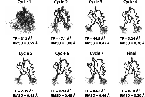
Semiautomated assignment of NOEs using simple chemical shift filters to suggest possible assignment combinations is an error-prone iterative process incompatible with a high-throughput structural proteomics pipeline. The NOEASSIGN module of the torsion angle dynamics (TAD) program CYANA provides a fully automated approach for the iterative assignment of NOEs (Guntert, Mumenthaler, and Wuthrich, 1997; Herrmann, Giintert, and Wui thrich, 2002b; Giuntert, 2004) that has performed robustly in our experience. Over the past 3 years, we have used NOEASSIGN to solve 14 unique structures by providing unassigned NOESY peak lists, dihedral angle constraints generated by TALOS (Cornilescu, Delaglio, and Bax, 1999), and a chemical shift list as input (Lytle et al., 2004a; Lytle et al., 2004b; Vinarov et al., 2004; Peterson et al., 2005; Waltner et al., 2005; Lytle et al., 2006; Peterson et al., 2006a; Peterson et al., 2006b; Peterson et al., 2007a; Tuinstra et al., 2007). NOEASSIGN uses the concepts of network anchoring and constraint combination (Herrmann, Gui ntert, and Wui thrich, 2002a; Gui ntert, Mumenthaler, and Wiuthrich, 1997; Guntert, 2004) in performing seven rounds of iterative NOE assignment with the result of the previous round used as a structural model (Figure 5.3). This automated routine enables the user to go from unassigned peak lists to folded structure in as little as 10-20 min, depending on the size of the protein and the available computational power (a 16 node/32 processor cluster was used here). NOESY peak assignments from NOEASSIGN are then verified or corrected manually using XEASY, and refined with additional CYANA calculations to generate a final structural model that meets basic acceptance criteria for agreement with experimental constraints, Ramachandran statistics, and coordinate precision.
Resolving Symmetric Dimers. A significant proportion of structural proteomics targets form stable oligomers in solution. Dimers and other oligomers with total molecular weight less than 30 kDa are amenable to high-through put NMR methods, and this highlights the need for an automated approach to solving structures of symmetric assemblies. CYANA supports automated structure calculations on symmetric homodimers and higher order oligomers. Dimeric proteins do not typically present a special problem for X-ray crystallography, but they offer a challenge for NMR methods because inter- and intramolecular NOEs are indistinguishable in uniformly 15N/13C-labeled samples due to chemical shift degeneracy between symmetry-related subunits. Thus, NOEs that define the dimer interface are not readily apparent in standard isotope-edited NOESY spectra. To identify intermolecular NOEs at the dimer interface, we prepare a differentially labeled sample by mixing equal amounts of unlabeled protein and uniformly 15N/13C-labeled protein and acquire a 3D F1-13C/15N-filtered, F3-13C-edited NOESY spectrum (Stuart, 1999). This spectrumcontains onlyNOEsarising between a proton directly bound to 13C nucleus and a proton bound to any NMR inactive nucleus while suppressing all other cross-peaks by isotope filtering. Constraints generated from the filtered NOESY spectrum can therefore be unambiguously assigned to protons on opposing faces of the dimmer interface.
Figure 5.3. Automated structure calculations using the NOEASSIGN module of CYANA. The structure of the second PDZ domain (residues 450–558) from Par-3 (PDZ2) was determined using the NOEASSIGN module of CYANA. Six files, including the sequence file, a chemical shift list, three unassigned NOESY peak lists with intensity values, and a list of dihedral angle constraints from TALOS were provided as input. The structural model in cycle 1 is generated based on chemical shift mapping, network-anchoring, and constraint combination. Continual improvements in the structural model are observed in the progression from cycle 1 to the final calculation as NOE assignments are verified and filtered against the previous structural model starting in cycle 2. The final structural model was defined by a total of 1,487NOE (759 short range, 199mediumrange, and 487 long range) and 117 dihedral angle constraints, and was completed in ~10 min using a 32 node cluster.
In theory, CYANA should be able to resolve the correct monomeric fold and dimmer interface from a combination of isotope edited and filtered NOE peaks when the MOLECULES DEFINE command is utilized in an NOEASSIGN run. MOLECULES DEFINE specifies the residue range for each monomer and works in conjunction with the MOLECULES IDENTITY and MOLECULES SYMDIST commands to minimize differences between torsion angles and distances, respectively, between corresponding atoms in the two monomers. Calculation of a symmetric homodimer requires the user to provide a sequence and chemical shift lists that contain explicit values for both subunits but only a single set of (nonduplicated) peak lists. Duplication of the symmetry-related NOESY distance constraints is performed automatically in NOEASSIGN when the MOLECULES DEFINE command is implemented. In our experience, NOEASSIGN fails to correctly define a homodimer unless ~20–30 intermolecular NOEs are manually assigned and maintained during the course of the iterative structure refinement. For example, 26 preassigned intermolecular NOEs were required for NOEASSIGN to converge to the correct structure forMZF1 (Peterson et al., 2006a). Once a structural model is obtained from NOEASSIGN, it can be used to seed a second NOEAS-SIGN run with all peak assignments reset at the beginning of the calculation. The second NOEASSIGN calculation typically generates more NOE constraints and a structural ensemble with lower root mean squared deviation (RMSD) and target function values when compared with the initial calculation. This ensemble is usually a suitable starting point for manual refinement in CYANA, final refinement in explicit water, or deposition in the PDB.
NMR Molecular Replacement Using CYANA/NOEASSIGN. As structural proteomics efforts increase the number of known folds and their representation in sequence space, the likelihood of finding a structural homologue for a particular protein increases. A 3D model of the target protein of interest may be generated from the structure of a likely homologue using MODELLER (Sali and Blundell, 1993) or other homology modeling programs. Inclusion of a homology model as a reference structure for the NOEASSIGN algorithm often improves the quality of the final model when compared with the results of a de novo calculation. In the early stages of iterative NOE assignment, knowledge of the global fold can provide a valuable distance filter that allows the selection of many unique distance constraints that would otherwise be treated ambiguously due to chemical shift degeneracy. We have applied this method to monomeric proteins with outstanding results, but the impact is even greater when applied to symmetric homodimers.
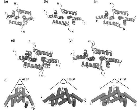
To solve the NMR structure of the homodimeric SCAN domain from ZNF24, we constructed a ZNF24 model (Figure 5.4a) based on the structure of tumor suppressor protein myeloid zinc finger 1 (MZF1; PDB ID 2FI2) (Peterson et al., 2006a). The model was included as a reference structure in an NOEASSIGN calculation performed on completely unassigned NOESY peaklists. The ensembles generated by NOEASSIGN converged to a domain swapped dimeric assembly (Figure 5.4b) similar to that observed for other members of the SCAN family (Ivanov et al., 2005; Peterson et al., 2006a). Consequently, the ZNF24 dimer structure was solved in much less time than the MZF1 structure.
Protein crystal structures solved by molecular replacement methods are susceptible to systematic error due to model bias, and it is important to assess the extent to which NMR refinement may be biased by areference structure. In contrast to crystallography, NOE-based refinement appears relatively insensitive to and unconstrained by the orientation of different structural elements in a seed model. Model-based filtering of NOE assignments relies on coarse estimates of interatomic distances for the initial round of refinement only, and is insensitive to long-range differences between the reference model and the true structure of the target protein. Consequently, the NMR analogue of molecular replacement may be more robust than the crystallographic version. To illustrate this point, we compared the NMR structure of the ZNF24 homodimer calculated using NOEASSIGN with the reference model created with MODELLER from the MZF1 structure (Figure 5.4d) and with an X-ray crystal structure of ZNF24 (Figure 5.4e). The reference model and the structure produced by NOEASSIGN exhibited clear differences in the overall arrangement of structural elements, suggesting that this method does not introduce a significant structural bias. Moreover, the NMR structure agrees very closely with the X-ray structure (Figure 5.4c), which was solved independently using phases obtained from single-wavelength anomalous dispersion, providing additional evidence that the automated NOEASSIGN algorithm converged on the correct structure for ZNF24.
Figure 5.4. Automated structure calculation of the ZNF24 SCAN homodimer using a seed model. (a) Seed model (green) of ZNF24 constructed using MODELLER software and theMZF1SCAN domain structure (PDB 2FI2). (b) NMR structure (magenta) of ZNF24 generated using the NOEASSIGN module of CYANA and the ZNF24 seed model shown in panel a. The NMR structure is defined by 2595 NOEs and 134 dihedral angles per monomer. (c) X-ray structure (cyan) of ZNF24 solved by single-wavelength anomalous diffraction using a mercury derivative. (d) Overlay of the ZNF24 model (green) and the NMR structure determined using the NOEASSIGN module of CYANA. (e) Comparison of the NMR and the X-ray structures. (f) Side view of all three models showing the change in the angle between helix 5 from each monomer as the seed model of ZNF24 is refined by NOEASSIGN to fit the experimental data. The more than 40° difference in the helix 5 angle between the seed model and the finalNMRstructure of ZNF24 suggests that the seed model does not bias the structure calculation. This is supported by the close agreement in helix angle when the NMR and Xray structures are compared. The figure also appears in the Color Figure section.
Final Refinement
The final stages of refinement often require inspection of NOE assignments that
result in consistently violated distance constraints. NOEs that have overestimated intensities due to
peak overlap can produce too restrictive constraints and require manual adjustment. A fully automated
refinement scheme may be able to resolve many such conflicts, but manual intervention is typically
required at some point to achieve the desired goals for precision (backbone RMSD below ~0.6Å), agreement
with experimental constraints (none violated by more than 0.5 or 5Å), and good torsion angle geometry
(no residues in disallowed regions of /ψ
space). CYANA provides diagnostic output with concise summaries of all the necessary data for each
ensemble of structures calculated, often simplifying the search for problematic restraints or
assignments.
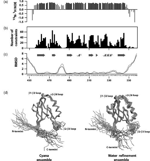
Average constraint density is an informative parameter that typically correlates with coordinate precision. NMR structures defined by more than 15-20 nontrivial constraints/ residue typically exhibit high coordinate precision, with RMSD values of 0.5-0.7 A for backbone atoms and 1.0-1.2 for all nonhydrogen atoms. However, it is also important to assess the local mobility of the polypeptide backbone using 15N relaxation measurements, since flexible regions will often be devoid of long-range NOEs. For example, 1H-15N heteronuclear NOE values show that most residues of a PDZ domain are ordered but an internal loop and both termini are flexible on picosecond-nanosecond timescales (Figure 5.5a). Consequently, the local NOE constraint density is expected to be low (Figure 5.5b), and no extra effort should be made to identify long-range NOE constraints for those residues. Automated NOE assignment algorithms may incorrectly identify long-range distance constraints for flexible residues, and these assignments can be rejected based on the evidence of local disorder provided by 15N relaxation measurements. Atomic coordinate precision, as reflected in local RMSD values (Figure 5.5c), mirrors the local constraint density, and this local flexibility is illustrated by the structural ensemble (Figure 5.5d).
When a complete and consistent set
of experimental constraints has been obtained, and the resulting structural ensemble meets the basic
acceptance criteria, a final refinement calculation is performed in explicit water with physical force
field parameters. A method for Cartesian space molecular dynamics in explicit water using XPLOR-NIH was
shown previously to improve the stereochemical quality of NMR structural ensembles generated with simple
force fields consisting only of terms for covalent geometry, experimental constraints, and a simple
repulsive potential (Linge et al., 2003). This conclusion was reinforced through the recalculation of
structures for over 500 proteins from standardized sets of restraints (Nederveen et al., 2005).
Improvements in a variety of validation criteria were observed upon water refinement of NMR ensembles,
particularly for the percentage of residues in the most favored region of the Ramachandran ( /ψ) plot. Systematically poor Ramachandran
statistics for NMR structures calculated with simplistic force fields can be attributed to the
unrealistic constraining of peptide bond planarity (w angle). In CYANA, for example, ω is fixed at 0° or
180°, corresponding to the cis and trans peptide
bond isomers. However, examination of high-resolution crystal structures in the PDB revealed a strong
correlation between the standard deviation of w and the proportion of residues
in the most favored /ψ regions. Consequently, relaxation of peptide bond rigidity during
water refinement in Cartesian space is accompanied by changes in and ψ, which improve overall quality of the backbone
conformation.
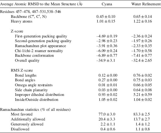
To simplify the water refinement routine, we have developed a script (available from BMRB) that converts the output of a CYANA calculation into input for water refinement and initiates the water refinement routine that utilizes a variety of software packages including XPLOR-NIH, CNS-SOLVE, PROFIT, PROCHECK-NMR, WHAT IF, and AQUA. While this routine is not fully integrated into CYANA calculations, the user can initiate a water refinement run with this single script once a complete and consistent set of experimental constraints has been achieved. Starting from the CYANA calculation directory, the script first creates a validation directory with a standardized structure and copies the required output files from CYANA to the validation directory. The CYANA files are then modified to ensure that residue naming conventions and numbering are compatible with the water refinement routine. Specialized input files that specify disulfide bonds, metal centers or cis-peptide bonds are also copied to the appropriate location during the initial setup. The script then initiates the validation run by parsing the input data and converting the distance and dihedral angle constraints into the XPLOR format. The initial structural model from CYANA is analyzed against the distance and dihedral angle constraints using WHAT IF and PRO-CHECK-NMR. The structural model is then refined using restrained molecular dynamics in explicit water using XPLOR-NIH as described above. Finally, the refined structural model is verified against the distance and dihedral angle constraints as previously described. A comparison of the input and refinement statistics shows that the Ramachandran statistics of the torsion angle dynamics ensemble from CYANA and the WHAT IF RMS Z scores are systematically improved by refinement in explicit water (Table 5.2).
Figure 5.5. Refinement and validation of structural models. (a) Heteronuclear 15N-1 H NOE values for the second PDZ domain from Par-3. NOE values below 0.7 are shown in light gray. (b) NOE distance constraint density plotted by residue number. Distance constraints used in the final structure calculation were derived from 3000 assigned peaks observed in three 3D NOESY spectra. Elimination of redundant NOEs and meaningless constraints (distances that impose no conformational restriction or are held fixed by covalent geometry) yielded a final set of 1222 NOE distance constraints. Including dihedral angle constraints from TALOS, a total of 1339 NOE and dihedral angle constraints were used in the structure calculation corresponding to ~12 restraints per residue. However, if residues with 15N- 1H NOE values below 0.7 are excluded from consideration, the restraint density increases to ~17 restraints per residue. Structures defined by <10, 10-15, and >15 constraints per residue typically correspond to low, medium, and high-quality structures, respectively. (c)The root mean squared deviation for the structural ensembles before (green line) and after (orange line) water refinement in explicit water plotted as a function of residue number. (d) Structural ensembles produced in CYANA using NOEASSIGN before (left panel) and after water refinement (right panel) show differences in conformational sampling for flexible loop regions as reflected by increased RMSD values in panel c. The helix, strand and loop elements in each ensemble are colored cyan, magenta, and salmon, respectively. The figure also appears in the Color Figure section.
Validation and Assessment of Structural Models
The optimal validation approach to be taken depends on the experimental data collected and how they were used in deriving the family of conformers that represents the structure. Two approaches are used for the validation of biomolecular NMR structures. In the first, the agreement between experimental data and coordinates is assessed. The second measures the match between many aspects of the geometry and the expected range of permissible values for each geometric parameter. Ranges of expected values can be derived theoretically or can be obtained from databases of protein structures (such as PDB), nucleic acid structures (such as NDB), and small molecules (such as Cambridge Structural Database, CSD). These types of structure validation provide complementary checks on the quality of structures and are described below along with various existing software packages.
TABLE 5.2. Structure Statistics for PDZ 2 of Mouse Par-3 (Residues 450-558)
As with X-ray structures, the stereochemical quality of protein models can be checked with the software tools PROCHECK (Laskowski et al., 1993) and WHAT IF (Vriend, 1990). NMR specific tools include AQUA and PROCHECK-NMR (Laskowski et al., 1996). Recently, WHAT IF has been extended to include a check on hydrogen geometry (Doreleijers et al., 1999b). Structural studies on peptides (Engh and Huber, 1991) and nucleic acids (Parkinson et al., 1996) solved at high resolution and present in the CSD resulted in a set of reference values and standard deviations of bond lengths and angles for heavy atoms that are taken as reference values for larger biomolecules. In most common force fields, the force constants for geometry constraints are chosen to reflect the variation in these geometric parameters. The check on bond lengths and angles is one among the various checks that should be performed before accepting a refined model. Severe deviations from the commonly accepted standard geometry signal the problematic regions in a structure.
Software packages used to solve and refine NMR structures (X-PLOR, CNS, DYANA, AMBER, and others) provide a rich set of diagnostic tools and a summary of the violations between the experimental data and the coordinates. Structures uploaded at deposition through the ADIT-NMR system can be checked using PROCHECK (Laskowski et al., 1993) and MAXit (Berman et al., 2000a). A number of additional software tools are available for evaluating the quality of derived NMR structures. Many of these can be downloaded from the World Wide Web or are available as web servers. These include Verify3D (Bowie, Luthy, and Eisenberg, 1991; Luthy, Bowie, and Eisenberg, 1992), ProSA (Sippl, 1993; Wiederstein and Sippl, 2007), MolProbity (Lovell et al., 2003; Davis et al., 2004; Davis et al., 2007), VADAR (Willard et al., 2003). WHAT IF (Vriend,) and AQUA (Laskowski et al., 1996; Doreleijers et al., 1999b). In general, NMR structures of acceptable quality meet the following validation criteria: (1) an RMSD for NOE violations less than ~0.05Å and no persistent NOE violation greater than 0.5Å across the ensemble of structures (Doreleijers, Rullmann, and Kaptein, 1998); (2) an NOE completeness of at least 50% for all NMR observable proton contacts within 4Å (Doreleijers et al., 1999a); (3) all torsion angles within the range of the restraints; and (4) chemical shift values within acceptable ranges, unless verified independently. At the time the structures are released, full documentation of the structure and the experimental data, as described in the IUPAC publication “Recommendations for the Presentation of NMR Structures of Proteins and Nucleic Acids” (Markley et al., 1998), should be provided, as well as the reports generated by the software packages mentioned above.
A number of approaches to validate NMR structures against NOE restraints or peak volumes and against residual dipolar couplings have been proposed (Gronwald and Kalbitzer, 2004). Kalbitzer and coworkers have developed an improved software package for back-calculating NOESY spectra from structures that take into account relaxation and scalar coupling effects; this approach and an associated “R” factor offer a promising way of validating NMR structures (Gronwald et al., 2000; 2007). Brunger and coworkers have developed a complete cross-validation technique, in analogy to the free R-factor used in X-ray crystallography, which provides an independent quality assessment of NMR structures based on the NOE violations (Brunger, 1992). The free R-factors of different NMR structures are comparable only if the NOE intensities have been translated into distance restraints in exactly the same way. Montelione and coworkers have proposed a combined scoring system for assessing the quality of NMR structures (Huang et al., 2005). The groups of Clore (Clore, Gronenborn, and Tjandra, 1998) and Bax (Ottiger and Bax, 1999) have developed a quality factor for residual dipolar couplings. In cases where dipolar coupling data can be obtained easily, this provides an attractive approach. A chemical shift validation quality factor also has been proposed (Cornilescu et al., 1998).
Validation of structural models against assigned chemical shifts is another promising technique for checking structures. The measurement of chemical shifts is easy and precise but the back-calculation of the expected chemical shift from a structure is less trivial (Case, 1998). Williamson and coworkers have related measured proton chemical shifts of proteins to values calculated on the basis of NMR and X-ray structures (Williamson, Kikuchi, and Asakura, 1995). The chemical shifts derived from NMR structures showed the same degree of agreement with the measured proton chemical shifts as X-ray structures with a resolution between 2 and 3 A(o of 0.35 ppm). Methods for back-calculating chemical shifts from structure are improving rapidly (Case, 2000; Xu and Case, 2001; Neal et al., 2003; Zhang, Neal, and Wishart, 2003). In addition to the AVS software tools (Moseley, Sahota, and Montelione, 2004), BMRB uses the linear analysis of chemical shift (LACS) (Wang et al., 2005) software application and chemical shift back-calculation routines in NMRPipe (F. Delaglio, unpublished) to validate assigned chemical shift depositions.
Deposition of Completed NMR Structures
Deposition of coordinates, chemical shifts, and structural constraints in public databases requires extensive data formatting and the entry of multiple kinds of information. In an effort to accelerate the deposition of new structures and improve the informational content of the entries, the PDB developed the AutoDep Input Tool (ADIT), a tool that accepts formatted input files using an expanded form of the macromolecular Crystallographic Information File (mmCIF) dictionary (Bourne et al., 1997; Berman et al., 2000b) or files in the PDB format. An mmCIF contains all the required structural data and experimental information needed to complete the deposition and automatically populates the query fields when parsed using ADIT. The BMRB in collaboration with the PDB used this system in developing a one-stop deposition system based on the NMR-STAR dictionary (ADIT-NMR; http://deposit.bmrb.wisc.edu/bmrb-adit/). This system is now available for submitting NMR-derived atomic coordinates, restraints, and all other experimental data to the PDB and BMRB. This interface, which can be accessed from the Research Collaboratory for Structural Bioinfor-matics (RCSB), Protein Data Bank (PDB), PDBj, or BMRB, minimizes the time required to complete the deposition to both data banks by allowing the user to upload and answer all queries once. The PDB takes responsibility for annotating the coordinates, and the BMRB takes responsibility for annotating the NMR data and restraints. The EBI is developing a new deposition system, but currently uses the older AutoDep system for structure depositions.
Generation of the mmCIF file can be conducted in either a semiautomated or manual fashion using the PDB_extract software available from the PDB website (Yang et al., 2004). This software extracts critical structural and experimental information from the output and log files generated by the programs commonly used in NMR and X-ray structure determination and combines it with the structural coordinates to generate a single file for upload. The resulting file can then be verified and/or edited manually to ensure that all information has been captured correctly prior to upload through the ADIT-NMR system. Alternatively, a template file generated by PDB_extract for NMR structures can be edited manually to include all the relevant information for the deposition of a particular target and passed to PDB_extract with the structural coordinates to assemble the mmCIF required for deposition. Our protocol calls for deposition of completed structures using a manually edited template file in conjunction with a script (available from BMRB) that automates the preparation of the final structural ensemble, distance and dihedral angle constraints, and chemical shift list for deposition. The script generates a single file containing both the distance and the dihedral angle restraints and runs PDB_extract to generate an mmCIF that can be uploaded to the PDB and BMRB data banks using the ADIT-NMR interface after a final review for accuracy. After the mm CIF, constraints file, and chemical shift list are uploaded to ADIT-NMR, the depositor must answer only few queries to complete the deposition to both databases. In our experience, this approach is considerably faster and more reliable than performing each structure deposition by completing all fields of the ADIT-NMR form via the web interface.
PROBABILISTIC APPROACHES AND AUTOMATION
Since the 1980s, the field of automated NMR analysis has been making strides toward a sound algorithmic foundation. A great deal of thought has gone into modeling the “analysis pipeline” (Figure 5.6). The principal aim of automated analysis is to ensure that the performance is satisfactory, or nearly optimal, even when there is uncertainty about the underlying data. The general approach has been to assume that the protein structure can be described as a bundle of conformers that satisfy an empirical force field and structural constraints. Variation in the conformers arises from uncertainty in the data, with large variations possibly indicating errors in prior steps in the pipeline (such as peak assignments orambiguity inNOEassignments) thatcouldbe “corrected” so as to lead to atighterbundle ofconformers. Overtime, itbecame clearthatsuchan approach can lead to overconstrained bundles. The reason is that in this model of uncertainty, every resonance assignment, experimentally derived restraint, bundle of structures, or protein residue in the sphere of uncertainty is deemed to be equally likely at each stage, and the decision is reduced to a binary accept/reject of observed data for use in the subsequent stage. Under such conditions, and combined with the incompleteness of the NMR experimental data, the algorithm is therefore obliged to guarantee equally satisfactory performance for every residue of every bundle within this sphere of uncertainty, irrespective of the level of uncertainty that may exist within the context of a specific NMR experiment and the specific protein under consideration.
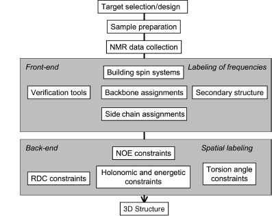
Figure 5.6. The standard pipeline for NMR structure determination consists of a number of discrete tools that, in reality, are intertwined by iterative cycles involving the detection and correction of errors. The front-end of NMR analysis is mostly concerned with “labeling of frequencies” derived from spectra while the back-end focuses on “spatial labeling.” Normally, the front-end and back-end are part of separate analyses; but ideally they should become part of a single analytic process.
Inherent uncertainties and incompleteness in experimental data as well as errors in modeling approximations (e.g., force field definitions) can lead to errors in attaining the correct fold or bundle of conformers. In short, NMR structure determination is a noisy, inverse, and ill-posed problem. In automating protein structure determination, it is particularly essential to carefully consider issues arising from uncertainties, including ways to explicitly measure and report them, because their impact can be remarkably difficult to detect otherwise. Errors can be broadly classified as either random or systematic. Random errors, often referred to as noise, lead to increased variance in results. In the language of robust analysis, noise is generally thought to have its largest impact on the reliability of results, but not necessarily on their accuracy. Systematic errors are usually more difficult to detect by computational methods, and they typically affect the accuracy of the results. To deal with sources of error and to address challenges faced in the traditional design of the pipeline, a recent approach has been adopted to include some notion of weight to the uncertainty in the databy assigning aprobability to results from each discrete step and to each subset of data. Thus, instead of assuring equally satisfactory performance at every possible residue or for every nucleus, the aim becomes to maximize the expected value of the performance of the algorithm. With this reformulation, there is reason to believe that the resulting model structures will better reflect the uncertainties in data than those based on deterministic uncertainty models.
The prospects for carrying out a fully probabilistic, automated program for NMR structure determination have been bolstered by advances in theoretical areas, such as algorithms that exploit relationships between local statistical potentials and global characteristics. It is now understood that global phenomena that obey a certain (large) family of probability distributions can often be described, or reasonably approximated, in terms of local potentials. Conversely, a set of local potentials could lead to a global description given by the same (large family) of probability distributions. These linkages are based on the Hammersly-Clifford theorem (Hammersley and Clifford, 1971; Spitzer, 1971; Besag, 1974), which implies that the efficacy of approximations given by statistical potentials is intimately tied to the accuracy of the description of the local potential. To understand the behavior of a certain global model, its sensitivity to estimates, and the reliability and accuracy of solutions, we can use an approach that combines elements of statistical mechanics and statistical decision theory while relying on local potential descriptions (Chentsov, 1982; Janyszek and Mrugala, 1989; Ruppeiner, 1995), which seems promising.
In the following sections, we first discuss how probabilistic approaches to discrete steps in the NMR structure determination pipeline (data collection, peak assignments, secondary structure determination, and outlier detection) can achieve remarkably effective outcomes. Then, we demonstrate how iterative combination of information from these discrete steps can lead to increased reliability and improved accuracy. The final section discusses how probabilistic tools can be used to address the ill-posed, inverse problem of NMR structure determination.
Adaptive, Probabilistic Data Collection
One of the challenges in protein NMR spectroscopy is to minimize the time required for multidimensional data collection. An innovative approach to this problem, “high-resolution iterative frequency identification (HIFI) for NMR” (HIFI-NMR) (Eghbalnia et al., 2005a), combines the reduced dimensionality approach for collecting n-dimensional data as a set of tilted, two-dimensional (2D) planes with features that take advantage of the probabilistic paradigm. For 3D triple-resonance experiments of the kind used to assign protein backbone and side chain resonances, the probabilistic algorithm used by HIFI-NMR automatically extracts the positions (chemical shifts) of peaks with considerable time saving compared to conventional approaches in data collection, processing, and peak picking.
The HIFI-NMR algorithm starts with the collection of two-orthogonal 2D planes. In cases where1H-15N and1H-13C 2D planes are common to multiple experiments, they need only be collected once. The algorithm then moves to the list of experiments specified for data collection and starts with the first experiment. For this experiment, tilted planes are selected adaptively, one-by-one, by use of probabilistic predictions. A robust statistical algorithm extracts information from each plane, and results are incorporated into the online algorithm that maintains a probabilistic representation of peak positions in 3D space. The updated probabilistic representation of the peak positions is used to derive the optimal angle for the next plane to be collected. The online software predicts whether the collection of this additional data plane will improve the model of peak positions. If the answer is “yes,” the next plane is collected and the results incorporated into the evolving model; if the answer is “no,” data collection is terminated for the experiment. The algorithm then proceeds to next NMR experiment in the list to be done. Once all experiments have been run, the peak lists with associated probabilities generated directly for each experiment, without total reconstruction of the three-dimensional (3D) spectrum, are ready for use in subsequent assignment or structure determination steps.
In achieving the steps outlined above, the probabilistic algorithm in HIFI-NMR divides the 3D spectral space into discrete voxels on the basis of prior information: the number of expected peaks; the nuclei involved and their expected chemical shift ranges; and the data collection parameters. Next, an empirical estimate for the prior probability distribution of peak locations in the multidimensional spectral space is obtained. The resulting joint probability distribution estimated in this step signifies the probability of a peak’s existence in a specific voxel of the spectrum. Let Ppr(X) denote the prior probability for the presence of apeak at position X, where the elements of the vector X =(x1, x2, x3) represent the voxels in three-dimensional space. The initial step in the HIFI approach is to collect data for the two orthogonal planes (0o and 90o planes). For experiments involving 1H, 15N, and 13C dimensions (e.g., HNCO, HNCACB), the 0° (13C - 1H), and the 90° (15N - 1H) planes are collected and peak-picked. Because the 1H dimension is common to the two planes, the possible candidates for peaks in 3D space can be generated by considering all combinatorial possibilities for peaks in the two planes that have the same 1H chemical shift within a given tolerance. This generates many more candidates than actual peaks, but will include most, not all, real peaks. These candidate peaks restrain the prior probability space generated in the earlier step. At the end of this stage, P0(x) designates the new probability distribution that includes information gained about the probability space consisting of candidate peaks.
The next best tilted plane is determined by assuming that the candidate peaks have been observed on a plane at angle θ and by evaluating the information theoretic impact of this observation on the probability of the peaks. The measure of this influence is the divergence Sθbetween the initial probability P0(x) (probability at the initial or the 0th step) and the predicted probability after the impact of the projection at angle θ has been taken into account Qθ(x):
(5.1)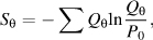
where the sum is taken over all voxels in the spectral space.
Next, each candidate peakx is examined in turn in the light of the data from the new tilted plane and prior data, and Bayes’ rule is used to update its probability P0(x) of being a “real peak,”
(5.2)
or
(5.3)
in which x_not_observed_in_θ is the complement event for x_observed_in_θ. The term in the denominator, P(x_observed_in_θ)orP(x_not_observed_in_θ) represents the probability of a voxel x in plane θ to be considered a peak (or not a peak), regardless of any other consideration. The probabilities P(x_observed_in_θ| x) and P(x_not_observed_in_θ| x)do not experience much angular variation and can be reasonably approximated by the empirical data. This process is continued until no significant information is obtained further. At this stage, n peaks with probabilities above a threshold are reported as the peak list. The value of n is estimated automatically from the number of amino acid residues in the protein, the type of experiment, and the probability distribution P(x). The value of n can be adjusted in a subsequent post processing step to include additional expert information regarding the data observed.
Probabilistic approaches are useful in a variety of situations where the robustness of analysis results needs to be validated. This includes the experimental determination of NMR coupling constants. HIFI-C (Cornilescu et al., 2007) represents the extension HIFI-NMR’s adaptive and intelligent data collection approach to the rapid and robust collection of coupling data. In this case, data collected from one or more optimally tilted 2D planes are used to determine couplings with high resolution and precision in less time than required by a 3D experiment. A further benefit of the approach is that data from independent planes provide a statistical measure of reliability for each measured coupling. Fast data collection can enable measurements in cases where sample stability is a limiting factor, as frequently happens with proteins in the orienting media used for determining reduced dipolar coupling data.
Probabilistic Approach to NMR Peak Assignment
Resonance assignment programs can be categorized by the methods they use in the mapping steps. These methods include stochastic approaches, such as simulated annealing/Monte Carlo algorithms (Buchler et al., 1997; Lukin et al., 1997; Leutner et al., 1998), genetic algorithms (Bartels et al., 1997), exhaustive search algorithms (Atreya et al., 2000; Andrec and Levy, 2002; Coggins and Zhou, 2003; Jung and Zweckstetter, 2004), heuristic comparison-based algorithms that predict chemical shifts derived from homologous proteins (Gronwald et al., 1998), and heuristic best-first algorithms (Zimmerman et al., 1994; Li and Sanctuary, 1997; Hyberts and Wagner, 2003). For example, AutoAssign (Moseley, Monleon, and Montelione, 2001) is a constraint-based expert system that uses a heuristic best-first mapping algorithm. Among these algorithms, those that rely on stochastic approaches have the best potential for satisfactorily addressing issues arising from noise.
In the PISTACHIO assignment algorithm (Eghbalnia et al., 2005b), the cost function is recast as a measure of “system energy” and the optimization problem is restated in physical terms as that of finding a “ground state.” This restatement enables one to ask questions that turn out to have tractable solutions with practical applications. For example, the approach makes it possible to ask for a “typical low energy configuration” and to find a computationally feasible (polynomial time) solution that gives a great deal of information about the “ground state.” This is pertinent to the NMR assignment problem because the available data may not support a unique set of assignments. An additional advantage to this approach is that it yields a set of assignment configurations with associated probabilities that can be explored and refined further as additional data becomes available. The local state of the statistical system is constructed in three steps. First, the peak list data are parsed into the set of all possible tripeptide spin systems and their associated scores. Next, tripeptides are assembled to match the sequence and to achieve the optimal probabilities for correct assignments. Each of the three steps serves to restrict the size of the combinatorial search space and to minimize the impact of noise on the analysis. The impact of noise is further ameliorated because the global ground state of the model corresponds to a state that is “statistically closest” to reported observations.
The starting point is to define a “local cost model” J(Y) in terms of a set of cost functions JN and their configurations YN that represent the spin system for a given tripeptide:
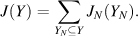
To minimize the overall cost J, one can maximize the following expression:
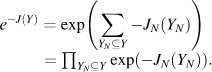
To treat this as a probability, a normalization factor is introduced,
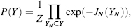
where the cost J is stated on the basis of pair-wise matching of tripeptides:
(5.4)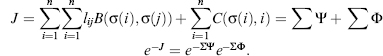
Upon dividing by the normalization factor to obtain probabilities, and by denoting the set of all permutations as S, the following expression is obtained:
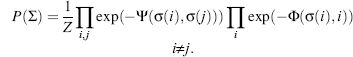
In Eq. 5.5, the second term measures the merit of assigning a tripeptide spin system Φ to a given tripeptide, whereas in the first term, ψ, provides a measure of the compatibility of the spin systems of adjacent, overlapped tripeptides. To achieve the goal of deriving probabilities for pairing spin systems with residues given by the Φ term, the marginal probability rather than the joint probability given by Eq. 5.5 must be calculated. One major practical advantage of this formulation is its generality because it does not rely on a specific experiment or set of experiments; rather, it enables an easy and efficient incorporation of data from multiple experiments into the framework. PISTACHIO is available as part of the PINE web server described below.
Probabilistic Secondary Structure Determination
Protein secondary structure plays an important role in classifying proteins (Lesk and Rose, 1981) and in analyzing their functional properties (Przytycka, Aurora, and Rose, 1999). Several algorithms have been developed for identifying secondary structure from NMR chemical shifts alone; these include the ∆δ method (Reily, Thanabal, and Omecinsky, 1992), the chemical shift index method (Wishart and Sykes, 1994b), the database approach by TALOS (Cornilescu, Delaglio, Bax, 1999), and the probability-based method (Wang and Jardetzky, 2002). A supervised machine-learning approachhas been used to combine data on sequence chemical shifts (Hung and Samudrala, 2003).
PECAN (protein energetic conformational analysis from NMR chemical shifts) is a probabilistic approach that utilizes a local statistical potential to combine the separate predictive potential of the sequence and chemical shifts in determining protein secondary structure (Eghbalnia et al., 2005c). Probabilistic and energetic models share some common ground through the Boltzman-Gibbs distribution. PECAN derives a residue-specific statistical energy function that is used to derive probabilistic secondary structure determinations. Suppose that wn is the number of observations of state n and En is the energy of state n. Further, assume that wn is approximately proportional to the probability for state n. Then, for a system in equilibrium in one of N possible states, the energy and probability are related as
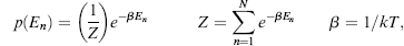
where k is the Boltzmann constant, T is the temperature, Z is the normalization factor called the partition function, and p(En) is the probability of state En. The constant β sets a monotonic scale for units of energy and can be set equal to a convenient constant. The energy term E is given by

Eq. 5.7 represents a finite model of length l, where the term Vi, represents the bias potential vector, which is determined by constructing optimized residue-specific density estimates that are related to energy through Eq. 5.6. Hj; j + 1 is a transition matrix for each state and represents the propensities of residues j and j + 1 to be in each of the possible state combinations. The values for the term Hj; j + 1 are derived from a database of experimental values. The two products Hj; j + j Vj and Hj— 1; j Vj represent two different stochastic mixings of the initial vector Vj. The parameter cj which can be replaced by a constant c, represents the proportional influence of the two terms and is optimized by reference to the database of experimental data.
Each site can be viewed as being in one of the three geometrically defined states: helix (H), strand (extended) (E), or “random coil” (R) (Figure 5.7). R is defined simply as neither H nor E. Each site has an associated energy that is coherent in the finite neighborhood l. For NMR chemical shifts of proteins collected under varying conditions of pH and temperature, PECAN yielded an average of 90% accuracy (93.5% helix, 83.5% strand, and 89.5% random coil) on a large data set (more than 85,000 residues). PECAN achieved a similar rate of success with a second set of data not previously considered (97 proteins; 12,000 residues). For 99% of the proteins, the identification accuracy exceeded 75%, and for 96% of the proteins, the accuracy exceeded 80%. PECAN is available from a web server at http://bija.nmrfam.wisc.edu/PECAN/ and also is incorporated into the PINE server described below.
Figure 5.7. Example of the use of the PECAN software to determine secondary structure from NMR chemical shifts and protein sequence (Eghbalnia et al., 2005c). The data are from BMRB entry 4083. The horizontal axis represents the sequence number. The vertical axis represents the probability of helix (gray), represented by positive values, and extended structure (black) represented by negative values. Values near zero indicate random coil residues. The white bars indicate the identification of regions without a discrete structural designation. Because a 3D structure of this protein is known (PDB 1CEY), the PECAN results can be compared with those derived from analysis of the protein conformation by DSSP (Kabsch and Sander, 1983), as shown at the bottom of the plot in cartoon representation where strands are arrows and helices are waves.
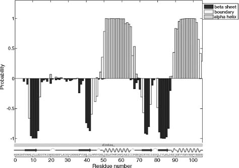
Validation
One validation approach that we have found valuable takes advantage of the finding
that, for a correctly referenced protein data set, linear regression plots of  versus
 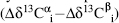 pass through the origin from two directions, the helix-to-coil and
strand-to-coil directions (Figure
5.8). Thus, linear analysis of chemical shifts (Wang et al., 2005) can be used to detect
referencing errors and to recalibrate the 1H and 13C chemical shift scales, if needed, and to recognize outliers that may indicate a possible misassignment or
abnormal backbone chemical shift. In the context of statistical potentials, the model of LACS assumes a
trimodal Gaussian distribution. LACS is available from a web server at http://bija.nmrfam.wisc.edu/MANI-LACS/.
pass through the origin from two directions, the helix-to-coil and
strand-to-coil directions (Figure
5.8). Thus, linear analysis of chemical shifts (Wang et al., 2005) can be used to detect
referencing errors and to recalibrate the 1H and 13C chemical shift scales, if needed, and to recognize outliers that may indicate a possible misassignment or
abnormal backbone chemical shift. In the context of statistical potentials, the model of LACS assumes a
trimodal Gaussian distribution. LACS is available from a web server at http://bija.nmrfam.wisc.edu/MANI-LACS/.
Figure 5.8. Example showing the analysis of assigned backbone 13Cαand 13Cβchemical shifts by the LACS algorithm (Wang et al., 2005). Data shown are for a single protein (BMRB entry 4998). The left-hand line represents the statistically linear trend of chemical shift values in α-helical regions and the right-hand line represents those for residues in β-sheet (extended) regions of the protein. Residues in nonhelical, nonextended regions are represented by points near the intersection of the two lines. This probabilistic analysis is useful for detecting possible misreferencing (as indicated by the deviation of the crossing point of the two lines from (0,0) expected for properly referenced 13C data) and for correcting the data so that the chemical shifts better represent secondary structure. The analysis can also detect outlier values that may represent misassignments or, as in the case shown (histidine, residue 56, indicated by arrow), a residue whose backbone carbon chemical shifts are pH dependent and thus not a reliable indicator of secondary structure. The probabilistic detection of outliers is depicted in the inset, which shows the normal distribution of points about the right-hand line.
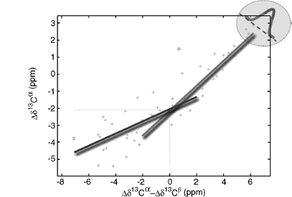
Integration of Probabilistic Steps within the Pipeline
The integration of individual probabilistic steps into a more global iterative analysis can be considered as the process of assigning a finite set of tags or labels to a collection of observations, subject to side conditions. This challenge is notable for its computational complexity and has theoretical and practical significance to a range of applications in bioinformatics. The combinatorial labeling paradigm is particularly problematic in modeling the early stages of NMR structure determination in which there is the need to associate amino acid labels, secondary structure labels, and other discrete attributes, to the observed data (NMR peaks with associated intensities and positions). The observed data often are incomplete and contain false positives and negatives. These characteristics render the robust assignment of labels remarkably challenging. The front-end labeling process associates one or more NMR parameters with a physical entity (e.g., nucleus, residue, tripeptide, helix, and chain); the back-end labeling process associates NMR parameters with constraints that define conformational states (e.g., dihedral angle, distance, and dipole orientation) (Figure 5.6).
One approach to carry out labeling in the presence of noise and incomplete data is cost function. For example, in the most straightforward case of using a chemical shift index to assign secondary structure, an entirely local three-state cost function was utilized (Wishart and Sykes, 1994a). Numerous cost functions of empirical or statistical nature have been proposed for problems ranging from assignment, secondary structure determination, dihedral angle restraints, to molecular dynamics force fields. Other approaches have used training algorithms, neural networks, or genetic algorithms. However, none of these approaches provides a principled answer to the questions of how many residues or resonances should be assigned, or how reliable and consistent such assignments need to be. To assign the best labels, the algorithmic process often optimizes additional parameters or introduces auxiliary criteria. As a result, it becomes necessary to introduce a variety of parameter setting rules, stopping rules, or other inspection methods. Often, validation tools are not utilized to test for systematic errors or outliers in the data, and no decision is tested against subsequent downstream decisions derived from experimental data (to ensure, for example, that the label from one step of data analysis is not in conflict with a label from another step).
A different view of labeling can be formulated within the context of information theory that explicitly implements the idea that NMR data analysis is motivated primarily by interest in some derived quantity (e.g., the protein structure) and that the solution strategy should focus on preserving information relevant to this goal, rather than trying to derive an optimal similarity metric in the local space of data. We imagine that each frequency label occurs together with a corresponding set of labels for the nuclei of a residue, along with additional labels indicating other information such as secondary structure state. In this formulation, there is no need to define a similarity measure; this measure arises from the iterative optimization principle itself. This approach is attractive because it frees us from the need to specify in advance what it means for the labels to be optimal. In addition, the basic idea can be extended with similar benefits to the entire NMR structure determination pipeline so as to identify in advance what it means for an NMR-derived structure to be most consistent with the data. Importantly, the approach enables the unbiased comparison of alternative algorithms for structure determination and analysis.
We have developed an algorithm called PINE that implements this approach to labeling and takes into account the interconnectedness of different stages of analysis (Figure 5.9). PINE begins with a set of local statistical potentials. It then proceeds iteratively until a stationary state for a consistent global similarity measure is achieved. The resulting software enables a seamless and robust integration of multiple steps in the NMR structure determination pipeline. PINE accepts combinations of NMR data specified by the user from an extensive list of NMR experiments, and provides as output a probabilistic assignment of backbone and side chain signals and the secondary structure of the protein. It also identifies, verifies, and rectifies problems related to referencing, assignment, or outlying data. PINE can make use of prior information supplied from selective labeling or spin system assignments derived independently by other means. PINE currently incorporates, and improves upon, the capabilities of PISTACIO, PECAN, and LACS. Extension of this core of algorithms can, in principle, support the additional statistical potentials involved in the back-end process of NMR structure determination.
Figure 5.9. Modeled relationships linking independent stages of evidence in protein NMR spectroscopy. The shaded ovals and solid lines indicate parts of the scheme currently implemented in the software package PINE (Bahrami, Markley, Assadi, and Eghbalnia, manuscript in preparation). PINE takes, as input, peak lists from different experiments, the protein sequence, information about labeling, and any prior assignments (used to override those determined). The analysis starts with an initial generation of an “almost exhaustive” list of spin systems in relation to the input data. The output currently gives backbone and side chain assignments and secondary structure. Future versions of PINE will work with longer range connectivities (from TOCSY and NOESY data) and, in addition, provide structural constraints (unshaded ovals and dotted lines).
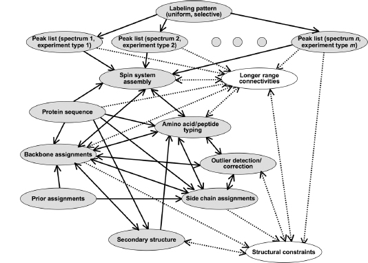
The input to PINE consists of the amino acid sequence and peak lists from one or more specified NMR experiments; the peak lists can be either probabilistic (e.g., peak lists generated by HIFI-NMR) or traditional types generated by popular NMR analysis tools. Starting with the spectral alignment step, which consists of a global and a local alignment, a probabilistic model is invoked. This can be viewed as assigning a distance probability for a peak i to belong to a spin system (SSj) as follows:
(5.8)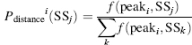
(5.9)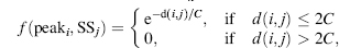
where d(ij) is the distance of the peak i and the reference peak in spin system j, and C is a constant that can be set to the resolution of the spectra (Lukin et al., 1997). In the spin system generation, nuclei of the spin system may have multiple chemical shift candidates with associated probabilities. Those probabilities can be derived from the distance probabilities described above along with the probability of existence of the peak itself (e.g., from HIFI-NMR-generated peak lists).
(5.10)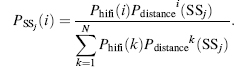
The total number of states of the spin system includes the combinatorial set of all nuclei choices, plus an extra state called null state. For the case of nonprobabilistic peak picking (traditional NMR experiments), the volume of the peak may be used to derive an estimate for significance of the peak to be used instead of Phifi. The preservation of all information at this step is particularly important for larger proteins where noise peaks and real peaks are closely interspersed in the spectral data.
The amino acid typing (scoring) step is the key in the integration of subnetworks. This process makes use of chemical shift probability density functions calculated from BMRB-PDB data for each atom of every amino acid in three states: alpha-helix, beta strand, and random coil. Amino acid typing is achieved by computing the probability of a chemical shift belonging to each residue i by
(5.11) 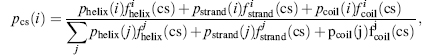
where 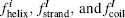 , are the chemical shift
probabilities of the related atom in amino acid i and phelix(i), pstrand(i), and pcoil(i) are the secondary structure probability
of the amino acid i with the condition
, are the chemical shift
probabilities of the related atom in amino acid i and phelix(i), pstrand(i), and pcoil(i) are the secondary structure probability
of the amino acid i with the condition
(5.12)
The above method connects amino acid typing and secondary structure states through a conditional dependency model. Notice that for the first iteration, where no assignment is available, secondary structure information follows a uniform distribution.
Deriving the backbone and side chain assignments from amino acid typing and other experimental data (connectivity experiments) is a computationally challenging element of the whole network. The approach in this step follows the model described in subsection, “Sequence-Specific Assignments.” First, the probabilistic assignments are analyzed by LACS for possible outlier detection. For each nucleus i and its assignment candidates j, one assigns a probability of being an outlier Py (outlier). Outliers need to be re-evaluated at each iteration. LACS also detects and corrects any possible referencing error in the spectra at this stage. Next, the PECAN algorithm (Eghbalnia et al., 2005c) is used to derive a probabilistic secondary structure determination. As the assignments are probabilistic (not unique), the combinatorial set of possible assignments and their corresponding secondary structures must be considered. After computing the probability of each residue i to be in each of three states (x = H, S, C) for different assignment configurations (c1, c2, cn), the overall probability can be calculated by
(5.13)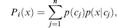
in which p(x|cj) is the probability of residue i to be in state x with the assignment configuration Cj, and p(cj) is the probability of the configuration Cj.
Posterior probabilities derived in the assignment process are used as prior probabilities in the next round of assignment, provided that (1) LACS has not flagged the assignment as an outlier, (2) the assignment is fully consistent with the predicted secondary structure, and (3) the assignment is consistent with established connectivities. If any of the above conditions does not hold, scores are re-evaluated in the next iteration. The iteration process continues until a stationary or quasistationary state is reached. The iteration process leads to “self-correction” through appropriate adjustments to the similarity metric to preserve maximum information. The integration of individual steps within PINE leads to results that surpass those achieved by stepwise application of the separate steps in the pipeline (Figure 5.10). Results from multiple automated analyses by PINE for a range of proteins demonstrate average assignment accuracies well above the level of 90% needed for subsequent stages of automation. PINE is available from a web server at http://pine. nmrfam.wisc.edu/.
Inferential Structure Determination
The back-end stages of structure determination involve the specification of three-dimensional coordinates for atoms of the macromolecule as derived from indirect observations in the earlier stages. In application domains where the forward model is very accurate and the numerical predictions of the model are in good agreement with the measurements, the procedure for dealing with noise and the sparsity of data is well understood. However, NMR data are noisy and sparse, and the forward model is insufficiently accurate to determine aunique structure. Thus, errors resulting from model misspecification can be significant. A common approach is to model these errors by including some “model-noise” and by regularizing the forward model to include restraint terms that enforce agreement with the observed data.
Figure 5.10. Representation of automated assignments determined for the protein ubiquitin from a set of input data generated by HIFI-NMR. The heights of the vertical bars indicate assignment probabilities. Correct assignments are indicated by green (high probability) and yellow (low probability) bars; incorrect assignments, as determined from the known structure, are indicated by red bars. (α) Results achieved by the PISTACHIO software package alone. (β) Results from the PINE software package. The comparison demonstrates the improvement in performance achieved by the multistep iterative probabilistic approach embodied in PINE (A. Bahrami, A. H. Assadi, J. L. Markley, and H. R. Eghbalnia, manuscript in preparation). Figure also appears in the Color Figure section.
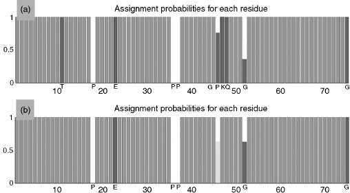
The current paradigm in NMR structure calculation is analogous to the process involved in inverting a noisy forward model. A typical scenario involves the minimization of a hybrid energy composed of an energy term representing the physical energy and a “regularization” term that measures the agreement of the model with the data through empirical measures. The components of the physical energy term describe the physical properties of the macromolecule, such as interactions between the atoms, and comprise the “force field.” The specification of the force field, however, does not sufficiently remove the degeneracy, and a regularization term is necessary to control the noise through agreement with the data. The degree to which this strategy works crucially depends on the quality of data. Specifically, when NMR structure determination is viewed as an ill-posed inverse problem, it becomes clear that the inversion strategy is successful if and only if the hybrid energy function does not describe a very rough energy surface. In cases where the hybrid energy represents a rough landscape, the determination of the weights for the regularization term becomes an expert’s task. In the absence of guiding principles, it is difficult to objectively evaluate the quality and reliability of determined structures. When structure ensembles depend on user-specific parameter settings and on the minimization protocol, statistically meaningful error estimates for atomic coordinates become practically infeasible.
Bayesian and maximum likelihood approaches have already proven useful for data analysis in NMR spectroscopy and X-ray crystallography. Intuitively, the uncertainties can be modeled by associating distributions to the parameter values that define the physical model of the protein. By replacing parameter values with distributions of values, and subsequently solving for a distribution of structure coordinates, the sensitivity of the structure coordinates to the parameters, and therefore the reliability of the resulting structure bundle, can be examined. This can allow the time (and space) evolution of the physical system to depart from deterministic evolution, thereby accommodating the effect of insufficiently modeled background events. For example, it is common practice to include the variance of the model-noise process in the collection of the parameters we wish to estimate from the data. It has been pointed out that allowing “model-noise” results in a good fit to the data, even if the deterministic part of the model is qualitatively wrong (Judd, 2003).
One approach to address the information insufficiency in structure determination is by amending the experimental data with some prior knowledge. Inferential structure determination views structure determination as an inference problem that requires reasoning from noisy and incomplete data (Cox, 1946). This approach does not lead to a unique structure; rather, it provides weights Pi for each conformation Xi —indicating the degree to which each conformation is supported by the experimental data. This inferential approach provides a principled way for handling the calculus of the inference problem (Cox, 1946; Jaynes, 2003). In this setting, the distribution of the probabilities Pi is interpreted as the information content of the data. A very sharp distribution of Pi values indicates a practically unique structure, while a flat distribution indicates lack of sufficient information for deciding among the conformational alternatives. The discrete setting can be readily generalized to the continuous model for the Cartesian coordinates of a macromolecule where probability densities now play the role of the probability mass. This Bayesian inferential approach demands that the probabilities be objective in the sense that they only depend on data D, and on relevant prior information I. The formal construction, through Bayes’ theorem, sets the posterior density to be proportional to the product of the likelihood of data given the model and the prior probability of a given macromolecular structure. This dependence on the prior is reflected in, for example, the use of the forward model; although other priors could be included. Other parameters that are required but cannot be measured, often referred to as nuisance parameters, are added to the list of parameters to be estimated. Therefore, the estimated density is formally a conditional probability that depends on the data D and the prior information I. This is a departure from the frequency view of probability.
In practice, the approach involves simulations of the posterior and sampling from areas of high probability mass. Once the terms in the Bayesian model have been established, the simulation provides an objective measure of agreement between data and the resulting structural model within numerical and simulation precision. Increased sampling of the conformational space and the suppression of entropically unfavorable states can provide a more realistic model of the macromolecule. The influence of parameters on the resulting model is transparent. For example, if the forward model does not incorporate any explicit information about protein dynamics, the formulation clearly shows that motion and imprecision due to experimental factors are indistinguishable. In addition, the sensitivity of the atomic positions to the parameters and the functional form of the force field can be explored in an objective manner.
It is often argued that the plausible specification of a prior is difficult or impossible. This difficulty can be addressed. Methods under development can achieve excellent results with little or no prior information. The robustified versions of these methods can guard against unexpected inferences resulting from prior selections. The current inferential approach focuses on the final stage of structure determination and does not rely on the propagation of uncertainties along the structure determination pipeline (Habeck, Nilges, and Rieping, 2005; Rieping, Habeck, and Nilges, 2005; Nilges et al., 2006). Although it is conceptually straightforward to include additional nuisance parameters, the increasing computational complexity and the presence of additional uncertainty models may lead to solutions that must be independently tested for stability and reliability. In the future, a comprehensive NMR pipeline based on inferential principles and capable of modeling other macromolecular features, for example, dynamics, should be capable of providing an objective, detailed, and feature-rich insight regarding the internal consistency, robustness, and accuracy of the resulting structural model.
DATABASES FOR BIOMOLECULAR NMR
The major international repository for biomolecular NMR data is Ulrich, et al., (2008), which is affiliated with the Research Collaboratory for Structural Bioinformatics (www.rcsb.org/) and is a member of the Worldwide Protein Data Bank (ww PDB, http://wwpdb.org/) (Berman et al., 2003). Coordinates for structural models derived from NMR data, as from crystallography, are archived at the Protein Data Bank (PDB, http://www.rcsb.org/pdb) (Berman et al., 2000).
Table 5.3 summarizes NMR data classes that are specific to biomolecular structure-function relationships. The primary information to be archived in a protein NMR investigation includes; (1) a complete description of the protein system studied (specification of each constituent and the stoichiometry of interacting constituents); (2) the solution conditions for each protein sample investigated (solvent, pH, temperature, pressure, and the concentration and isotopic labeling of each constituent); (3) a full description of each NMR experiment used in collecting data for the sample; (4) the NMR parameters and derived information obtained in the investigation; and (5) the unprocessed, time-domain NMR spectra collected. The present goal of the databases (PDB and BMRB) is to accommodate the inclusion of additional information on the preparation of the sample and the methods for structure determination at the level of detail provided in the methods section of a research journal. BMRB also accepts full data sets (time-domain spectra plus intermediate results) contributed by authors associated with a structure determination and now has archived more than 90 such sets to date.
In the interest of maintaining a common chemical shift standard for biomolecules, the international community has adopted the methyl signal of internal 2,2-dimethylsilapentane-5-sulfonic acid (DSS) at low concentration as the1H chemical shift standard. Chemical shifts of nuclei other than1H are referenced indirectly to the1H standard through the application of a conversion factor for each nucleus derived from ratios of NMR frequencies (Markley et al., 1998). The BMRB (Ulrich, Markley, and Kyogoku, 1989; Seavey et al., 1991) contains over 3.1 million experimental chemical shifts for proteins, nucleic acids, and small molecules as well as more than 14,000 experimental coupling constants. As of 2008, there were 2357 BMRB entries with associated PDB entries; of these, 1404 BMRB were available with chemical shifts referenced consistently using the IUPAC recommendations.
NMR structures in the PDB are represented by a description of the input data used for structure determination and refinement, the methods used to determine the structure, a statistical analysis of the results, and the structure itself, which usually is represented by a family of conformers that best satisfy the input constraints along with geometric and energetic criteria. One of these conformers is specified as being the single representative structure.
BMRB archives additional information about the chemical properties and dynamics of proteins derived from NMR spectroscopy, including hydrogen exchange rates at specified sites and pH titration parameters (pKa values, Hill coefficients, and pH-dependent spectroscopic shifts) for titratable groups and relaxation parameters (heteronuclear NOE, T1, T1rho, T2, and order parameters). Figure 5.11 illustrates the full range of information at BMRB.
TABLE 5.3. Summary of the NMR Data Classes That are Specific to Structural and Functional Genomics
NMR-STAR is the data model and tag-value data format for biomolecular NMR developed by BMRB in collaboration with the PDB, the Collaborative Computing Project for NMR (CCPN) (Fogh et al., 2002), and a number of contributors from the NMR community. NMR-STAR is an implementation of the STAR format developed for the communication of information in a compact ASCII format (Hall, 1991; Hall and Spadaccini, 1994). The mmCIF data dictionary and data format are STAR implementations used in biomolecular crystallography (see Chapter 10). BMRB has developed software tools for interconverting NMR-STAR and mmCIF. NMR-STAR is used by BMRB as its data input format and by many biomolecular NMR software packages as a data exchange format. Specification of the NMR-STAR format and software tools for operating on NMR-STAR files are available from the BMRB web site (http://www.bmrb.wisc.edu). BMRB data are exported in theASCIINMR-STAR format and in a format that can beloaded easily into a relational database.
Figure 5.11. Potential information content of aBMRBentry for a particular target (study) showing the interrelatedness of the data to be collected.
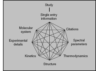
BMRB established two new databases of structural restraints used to calculate NMR structures: DOCR (Database of Converted Restraints) and FRED (Filtered Restraints Database) (Doreleijers et al., 2005). Both databases were constructed in collaboration with EBI and CCPN groups from restraint data available from the PDB. The DOCR database contains restraint files with atom nomenclature consistent with the nomenclature in the corresponding atomic coordinate files. The restraints data in the FRED database have been filtered to remove redundant values and other restraints that do not impact the structure calculations. Over 500 protein structures were recalculated using restraints from these databases and the resulting structures analyzed for their quality (Nederveen et al., 2005). The resulting database of recalculated structures (RECOORD) is available on the web (http://www.ebi.ac.uk/msd-srv/docs/NMR/recoord/main.html). The DOCR and FRED databases now contain over 4000 PDB NMR entries. The data are available in NMR-STAR format, X- PLOR, or an XML format.
As BMRB expands, the database of publicly accessible biomolecular NMR data also expands, creating a highly valuable resource for data mining and the development of statistical correlations between NMR observables and the structural and chemical properties of biomolecules. Examples include SHIFTY (Wishart et al., 1997), RefDB (Zhang, Neal, and Wishart, 2003), TALOS (Cornilescu, Delaglio, and Bax, 1999), AVS (Moseley, Sahota, and Montelione, 2004), PISTACHIO (Eghbalnia et al., 2005b), PECAN (Eghbalnia et al., 2005c), and other probabilistic studies (Wang, Eghbalnia, and Markley, 2006). BMRB routinely uses the AVS software package to inform depositors of suspicious or anomalous assigned chemical shifts within their depositions.
ACKNOWLEDGMENTS
We thank the members of the CESG, NMRFAM, and BMRB teams for their contributions. Support from NIH grants P41 LM05799, 1U54 GM074901, and P41 RR02301 is gratefully acknowledged.