8

SEARCH AND SAMPLING IN STRUCTURAL BIOINFORMATICS

Ilan Samish

The road was still paved with yellow brick, but these were much covered by dried branches and dead leaves from the trees, and the walking was not all good.

L. Frank Baum, in The Wonderful Wizard of Oz, 1900.

INTRODUCTION

Search and Sampling—Tools of Structural Bioinformaticians

Structural bioinformatics aims to gain knowledge about biological macromolecules utilizing computational methods applied to structural and structure-related data (see definition in Chapter 1). Search and sampling methods aim at providing a focused “yellow brick road” toward understanding the properties of complex biomolecular structures. Such methods must often be tailored for this unique field. First, intrinsic to the “bio” nature of the data is high complexity in the number and the type of variables. Structural data is derived experimentally from various sources and is presented in different resolutions (Chapters 2-6). Moreover, other types of data often need to be integrated in the processing of structural data. These include (1) the exponentially growing sequence data, for example, in the form of evolutionary conservation (Chapters 17, 23, 26), as well as (2) biophysical data, for example, stability of proteins, distance restraints between residues as derived from mass spectroscopy (Chapter 7) or analysis of mutational data. Second, the required representative space (defined later in the chapter) one wishes to study is often biased, not fully covered or cannot be fully sampled. Scientific research tends to produce focused data on specific regions, rather than, unveiling the full space. Third, often the available data types or the integration of data from different sources requires specialized search and sampling. Since the physically based rules governing the behavior of biological macromolecules are still not fully understood, or may be not practical to compute, phenomenological data are often utilized. In the resulting “knowledge-based” parameterization, the interplay between the constituting variables need not be fully understood to be useful. Yet, the generality of such parameterization and the correlation between resulting parameters have to be addressed. Finally, with the diminishing boundaries between structural bioinformatics and computational biophysics, the former may expand in scope by adding more data as well as new complex variables, for example, the fourth dimension of time. Notably, these required factors for search and sampling are evident whether studying a single macromolecule, an ensemble of related macromolecules, or a (sub) space of structural data.

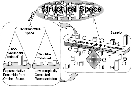
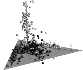
The process of structural bioinformatics search and sampling methods can be divided into several general groups or steps. First, the sampling stage seeks to ensure that the “answer space” of the assessed question is properly covered. Second, the search stage sets to select the important and relevant information within the vast available data. As shown in Figure 8.1, these two stages are intimately entwined. Third, the analysis stage deals with inferring the biological meaning of the data, and as a result the data can often be classified into few or numerous divisions. Finally, the optimization and quality assurance stage examines the analyzed data with its related quality and chooses the most correct answer. Alternatively, this stage may result in a decision to conduct further fine-tuning analysis, reduce the data derived from the search space, or even go back and revise the sampling process. While the latter two stages are an integral part of the search and sampling process, here we will focus on the first two stages.

The methods of search and sampling structural space comprise a broad group of tools essential to numerous structural bioinformatics applications. In this brief chapter, we cannot exhaustively cover the mathematical foundations associated with these methods, nor their numerous structural bioinformatics applications. A short introduction of terms and philosophy is introduced in the following section. Further description of such techniques can be found in other sources relating to (1) general methods, for example “Monte Carlo applications in science” (Liu, 2001) or “Markov chain Monte Carlo in practice” (Gilks et al., 1996), (2) bioinformatics from a machine learning approach (Baldi and Brunak, 2001), and (3) structural bioinformatics and computational biophysics books (Becker MacKerell et al., 2001; Leach, 2001; Schlick, 2002). Here, we aim to present the rationale behind some of the different algorithms along with their advantages, limitations, and examples of applications to structural bioinformatics research. The chapter opens with a brief introduction to Bayesian statistics, which is the underlying formalism and rationale to most methods developed in this field. Indeed, some of the studies cited in this chapter utilize the Bayesian formalism explicitly (e.g., Simons et al., 1997; Dunbrack,; Dunbrack, 2002), while others follow the Bayesian rationale despite not being presented through this formalism. Next, some of the major methods and applications for representative sampling and search of conformational space are described. As a concrete applicative example and without losing generality, we focus on the classic challenge of exploring conformational space of proteins, mainly at the side-chain level.

Underlying Terms: From Frequentist (or Sampling) Statistics to Bayesian Statistics

A very basic introduction to the underlying terms and a way of thinking as it relates to statistical fundamentals of search and sampling is essential. Statistics was presented in the 18th century for the analysis of data about the state (statisticum in Latin is “of the state”). Within the broad quantitative examination “of the state,” more than one approach was developed. Frequentist statisticians focus on having methods guaranteed to work most of the time, given minimal assumptions. The probability is given only when dealing with well-defined multiple random experiments. Each experiment can have only one of two outcomes; it can occur or it does not occur. As a random experiment, there is no a priori knowledge that will bias our knowledge on the outcome of the experiment. Note, as the set of all possible occurrences is often called “sample space,” frequentist statistics is often referred to as “sampling statistics.” However, here we will not use this term to avoid confusion. Contrary to frequentist statistics, Bayesian statistics (also known as Bayesian inference) attempts to make inferences that take into account all (or all “relevant”) available information and answer the question of interest given the particular data set. The observations are used to update, or newly infer, the probability that a hypothesis may be true. The degree of belief in the hypothesis changes as the evidence is accumulated. A debate still exists between the two methods, often resulting from misleading interpretations of common statistical terms (MacKay, 2005). In most but not all structural bioinformatics studies, Bayesian statistics is the method of choice (Dunbrack, 2001).

Formally, frequentist statistics deals with a function, also called statistic, S, of the data, y. The statistic is a summary of multiple occurrences, N, of a specified experiment obtained from repeated trials. A hypothesis, H, about the data is tested as true or false. Thus, the hypothesis cannot have a measured likelihood or probability but rather can be accepted or rejected. Most often the null hypothesis that is at odds with S(y) is utilized with the overall objective of rejecting it. The null hypothesis is rejected if the probability of the data is small (e.g., less than 5%) given the truth of the hypothesis. This requires a comparison of the statistic of the observed data (also called actual data) to the distribution of all possible (and usually simulated) data p(S(y_simulated)|H). Thus, if ∫^∞S(y_actual)P(S(y_simulated)|H)d S(y_simulated) < 0.05, then the null hypothesis can be rejected. The probability distribution and its associated quantities such as the variance σ² are defined in terms of parameters θ that may be inferred from the data. Confidence intervals can be defined as the range of parameter values for which the statistic S, such as the, average,y, would arise 95% of the time. For example, a 95% confidence interval for the mean θ (for normally distributed data) is obtained as follows:

(8.1)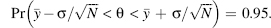

Unlike frequentist statistics, probability in Bayesian inference is the degree of belief in the truth of the statement. For example, in confidence interval terms, this would mean the probability of the parameter given the data, rather than the probability of the data given the parameter; that is,

(8.2)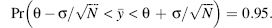

The probability of any hypothesis, H, is conditional upon the information, I, we have on the system, namely, p(H|I). The sum rule and the product rule form two basic rules upon which Bayesian inference relies. The sum rule states that given the information, I,we have on a system, the cumulative probabilities for a hypothesis, H,and its inverse, denoted H^y (note, this is the same common annotation used to denote average), to be true is equal to one, that is, p(H|I)+ p(H|I) = 1. The product rule states that the probability of occurrence of two hypotheses, or events, is equal to the probability of one event multiplied by the conditional probability of the other event given the occurrence of the other event, namely, p(A,B|I)= p(A|B,I)p(B|I) = p(B|A I)p(A|I). As in all these probabilities the same information on the system is assumed, so “I” can be dropped from the equation resulting withp(A, B)= p(A|B)p(B) = p(B|A)p(A). In Bayesian inference, the probability of a hypothesis given the data is pursued. In the sum rule, event A can be replaced by hypothesis, H, and event B by the data, D, resulting in p(H|D)p(D)= p(D|H)p(H). Dividing both sides by the marginal distribution of thedataprovidesa waytomeasurethe posterior distribution—the probability of the hypothesis after examining the data. This distribution is expressed by Bayes’ rule (Bayes, 1763):

(8.3)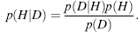

The prior probability, p(H), is of the hypothesis before considering any data. If the prior distribution may remain uniform over the entire distribution of the data, then the data are said to be uninformative, or if the distribution may be higher for some ranges of the data, then it is said to be informative data. In either case, it should be proper, that is, normalized to integrate to one over the entire data range. The likelihood of the data given that the hypothesis is true is expressed by p(DjH). Uncertainties in measurement and physical theory connecting the data to the hypothesis are expressed by this term. Finally, p(D) is the marginal distribution of the data—a quantity that should be constant with respect to the parameters and act only as a normalization factor.

Bayesian statistics is often applied to specific questions using Bayesian models in which prior distributions are computed for all parameters and a likelihood function formulized for the data given the parameters. Then the posterior distribution of the parameters is computed (analytically or via simulation) based on the data. Finally, the model fitness to the data is evaluated by utilizing posterior predictive simulations. Data predicted from posterior distribution should resemble the data that generated the distribution and be physically realistic.

While frequentist theory has an analytical power in quantifying error as well as differences between groups of data, Bayesian statistics is often more intuitive to scientific research. The very basic scientific way of thinking includes the use of the prior distribution and the focus on parameter value ranges for the data. The possible subjectivity of the Bayesian prior distributions was not accepted by early frequentist statisticians. Yet, the latter use test statistics calculated on hypothetical and often unintuitive data. Some see the subjective need for prior distribution in Bayesian statistics as an advantage. Importantly, the choice of the prior distribution requires considering the full range of possibilities for the hypothesis. Further, it is possible to consider varying degrees of informativity, including the possibility of coupling parameters from unrelated data. As a result, Bayesian statistics is often the underlying rationale for structural bioinformatics.

SAMPLING STRUCTURAL SPACE

Sampling of a space can be achieved by multiple random accesses to the space or by a continuous walk within the space. The ergodic hypothesis, described in the next section, presents the equality between both approaches. Whatever approach is utilized, accurate sampling should ensure proper coverage of the sampled space. A proper coverage includes a full coverage of the space under the given covering resolution and, complementary, the lack of focusing on one area within the space. Often, a representative set is built from the original space to achieve proper sampling. The next sections will describe the definition of the representative spaces in the full protein and in the side-chain hierarchy levels. Notably, when dealing with structural space with multiple local minima, for example, an energy landscape, often the best search is conducted by sampling the full space at low resolution and areas of interest at higher resolution. This important topic will be discussed under the “search” segment of this chapter.

Basic Terms: The Ergodic Hypothesis, Providing the (Detailed) Balance Between Thermodynamic and Dynamic Averages

The ergodic hypothesis is a basic underlying principle in structural bioinformatics and, more generally, in statistical thermodynamics. Historically, the word “ergodic” is an amalgamation of the Greek words ergon (work) and odos (path). The ergodic hypothesis claims that over a sufficiently long period, the time spent in a region of phase space of microstates with the same energy is proportional to the size of this region. In the context of structural bioinformatics, the phase space is often the energy landscape, that is, the energy of the investigated macromolecule(s) for each possible conformation. The hypothesis was first suggested by Ludwig Boltzmann in the 1870s as part of statistical mechanics. Neumann proved the quasiergodic hypothesis (Neumann, 1932), and Sinai gave a stronger version for a particular system. For a historical background as well as yet to be resolved aspects, see Szasz (1994).

For sampling algorithms, the ergodic hypothesis implies that after a sufficiently long time, the sampling algorithm makes an equal number of steps in different equal volumes or regions of phase space. In other words, the ensemble, or thermodynamic average, for a phase space region is equivalent to the time average, also termed the dynamic average. The thermodynamic average is defined as the average over all points in phase space at a single time point, while the dynamic average averages over a single point in phase space at all times. In this context, the assumption of equilibrium means that moving from state X to state Y is as likely as moving from state Y to state X —that is, the system obeys the detailed balance criterion. Utilizing biased techniques, the detailed balance may be violated but only if properly corrected to approach the requested description of equilibrium.

In the field of structural bioinformatics, detailed balance sets the stage for (1) studying structures using sampling of microstates, for example, via Monte Carlo (MC) simulations, (2) studying a dynamic analysis of a single trajectory, for example, molecular dynamics (MD), and even more importantly, (3) enabling the interchange between the two. Of course, any interchange between the two approaches depends on the accuracy of each method. This accuracy includes complementary aspects such as the size of phase space, the density of sampling the space, and the completeness of the sampling within the defined space. The completeness and the density of the sampling define the representativeness of the assessed phase space. For example, representative sampling is necessary to establish accurate thermodynamic averages as well as the phase space probability density, the probability of finding the system at each state in phase space. In MD, the spatial precision often required for accurate solution of the equations of motion necessitates a small time step for the trajectory propagation coupled with a simulation time that fits the assessed phase space. This is to ensure sampling of all the required phase space taking into account the need to overcome, directly or indirectly, local barriers in the rough energy landscape of the macromolecule. Often, while the local explored region, for example energy landscape, is fully ergodic, high-energy barriers prevent the sampling of distant low-energy regions. The quasiergodic sampling requires designated methods to overcome the challenging energy landscape architecture. Approaches to avoid this local minimum trap include raising the energy of the local low-energy basins, for example, accelerated molecular dynamics (Hamelberg et al., 2004), or the occasional high-energy jumping above barriers (presented below). Therefore, structural bioinformatics research must constantly address the aspect of ergodicity when drawing general conclusions from the limited available data.

Defining a Nonredundant Data Set for Representative Sampling of Available Data

To understand the structural (sub)space of proteins, one needs a representative description of this space. Even if the size of the space did not pose a limitation, which it often does, the large amount of redundant information will bias any requested underlying characterization of this space. In constructing a nonredundant representative structural data set, several aspects should be addressed. First, the multidimensional phase space should be defined. Second, low-quality noninformative data should be excluded. Third, and more difficult to implement, the data should be representatively distributed in phase space. Following the ergodic hypothesis, any general conclusions about a structural (sub)space should aim at utilizing data that equally samples the different parts of phase space rather than averaging all the available and intrinsically biased data. Thus, the derivation of a nonredundant structural space is a key step in the computational analysis of structural data.

Defining a Nonredundant Data Set in the Protein Structure Level. One possibility of characterizing structural (sub)space is to utilize available structural data and attempt to overcome the known limitations in the representativeness of the data. Here, we will use the Protein Data Bank (Berman et al., 2002) (Chapter 11) as an example of the challenges in creating a representative set. As shown in Figure 8.2, this database is naturally biased toward the focus of the research that generated it as well as the ease of generating the data. Well-represented proteins include medically relevant small proteins, historical “model proteins” that were crystallized under many conditions and modifications, and proteins from interesting creatures, for example, Homo sapiens. In contrast, some structures are underre-presented as they are technically hard to obtain. These include very large proteins, intrinsically mobile proteins, and membrane proteins.

How does one define, sample, and generate a representative nonredundant set? Prior to answering this challenge, the representative nature should be defined. The topic is especially relevant in the current age of structural genomics (Chapter 40), where the focus is to fill gaps and achieve a fully covered structural space. Typically, geometric and sequence redundancy are addressed. Other definitions for representativeness such as functional differentiation (Friedberg and Godzik, 2007) or a combination of classifiers such as secondary structure content, chain topology, and domain size (Figure 8.2) (Hou et al., 2003) were also suggested. Several “nonredundant” databases exclude redundant structures based on sequence identity. For example, the PDBSELECT database provides structures with low sequence similarity (Hobohm et al., 1992; Hobohm and Sander, 1994). The PDB search engine (Deshpande et al., 2005), PISCES (Wang and Dunbrack, 2005) and Astral (Brenner et al., 2000) allow for the creation of user-defined nonredundant sets utilizing user-determined sequence redundancy, resolution and other structural quality cutoffs.

A widely accepted automatically generated nonredundant database based on representativeness of fold space is still missing. This is partially due to the subjective definition of folds. Topics such as complexity, definition of redundancy, and representativeness of a subset have been addressed since the early days of the PDB. Fischer et al. built a sequence-independent nonredundant PDB resulting in 220 representative structures (Fischer et al., 1995). A less subjective definition of fold representativeness can by obtained by selecting representative structures from the different subgroups of the fold, as obtained from classification databases such as SCOP (Murzin et al., 1995), CATH (Greene et al., 2007), or DALI (Holm and Sander, 1996) (Chapters 17 and 18).

Protein structures can be represented by smaller units of structure (Chapter 2). The building blocks often comprise subunits of sequences or, in the case of structures, domains. The domain (Chapter 20) is classically defined as a group of amino acids within the protein structure that is stable to the point of folding independently from the rest of the protein. Domains often consist of all or part of one chain, but may consist of parts of different chains. Both types of building blocks are currently utilized, but consideration should be taken when deciding which strategy to use. On the one hand, it is easier to define and work with sequence information. On the other hand, the structural domain definition may be more accurate for some applications where structural folding units are addressed. Finally, the correlation between structures has to be addressed. For example, an independent distribution of structures must sample structure space without a bias toward a specific common ancestor of a subgroup within a given common “superfold.” The CATH-based Nh3D database addresses this important aspect (Thiruv et al., 2005).

Hence, while the importance of nonredundant structural databases is well established and while there are databases of nonredundant structures or means to compute such sets on-the-fly, the field is still evolving. With the increasing number and accuracy of available structures and unique domains/folds contributed by the structural genomics efforts, topics such as a proper definition of a structural phase space and the proper sampling of the defined space continue to be addressed.

Defining a Nonredundant Data Set at the Protein Residue Level. At the backbone level (Chapter 2), Φ and ψ are sufficient to describe the conformation of each residue in the protein chain. The Ramachandran plot that describes these angles exhibits distinct clustering that corresponds to the different secondary structures. Similarly, at the side-chain level, clustering the dihedral angles is an efficient method to describe conformational space. Figure 8.3 introduces the notion of rotamers. The dihedral angle between the C_α and C_β (namely, N-C_α -C_β-Xy(1)) Where X denotes atoms of type C, N, O, or S) is termed χ₁, the dihedral angle between C_α and C_β (namely, Cα-C_β-X_γ(₁)-X_δ(1)) is termed χ₂, and so on. The set of side-chain dihedral angles determines a single side-chain conformation termed rotational isomer, or rotamer (Dunbrack, 2002). Rotamers are not evenly distributed and represent local energetic preferences. Beyond the general preference for staggered conformation (60°, 180°, —60°), the backbone conformation limits the side chains to specific conformations.

Computational efficiency may be achieved through better data representation. Working with a rotamer library that defines the average dihedral angles for the most common rotamer clusters for each residue helps to reduce the dimensionality of the data. This has a dramatic effect as often such data have to be accessed multiple times. Other efficient structural data processing schemes, for example, geometric hashing (Nussinov and Wolfson, 1991), also make use of preprocessed data that can later be efficiently accessed. In the case of rotamer libraries, the transformation to dihedral space forms an additional measure of data reduction. The transformation assumes an idealized (within error) covalent geometry. The resulting rotamer library can be viewed as a look-up table that allows the user to process structural data within a more manageable structural space.

Early studies utilized as few as 84 rotamers to represent the 19 side-chain conformations (Ponder and Richards, 1987). More recently, others constructed very large libraries with as many as 50,000 rotamers (Peterson et al., 2004). Holm and Sander have shown that in most cases increasing the library size does not improve our ability to identify the global low-energy solution (Holm and Sander, 1992). Rotamer libraries provide the relative frequency of each rotamer, providing an additional level of information. Rotamers that are not described in the library are denoted as “non-rotameric” conformations. In general, rotamers fall within well-defined statistical bounds. Yet, in specific regions, for example functional sites, rotamers may define unique conformations. These rotamers are often stabilized by a specific set of interactions to other protein or cofactor moieties. Therefore, by simply examining the distribution of rotamers in the protein, functional insight can be deciphered.

Importantly, the accurate representation of a rotamer library highly depends on the accuracy of the raw data applied. For example, Richardson and coworkers (Lovell et al., 2000) filtered the data in several ways: Beyond the selection of high-resolution proteins (resolution better than 1.7Å) other structural quality assurance (Chapters 14-15) filters were applied: Side chains with high intrinsic thermal motion (as marked by B-values greater than 40A) were removed. Likewise, side chains that exhibit steric clashes after properly adding hydrogens to the heavy atoms were not included and side-chain flipping was applied to residues (Asn, Gln, and His) that were not modeled correctly in the original PDB file. This led to improvement in the resulting rotamer library and underscores the need to examine raw data very carefully prior to drawing conclusions. An alternative approach is to move from the coordinate data to the source electron density data and eliminate residues with poor density (Shapovalov and Dunbrack, 2007).

Rotamer libraries can also depend on the backbone conformation, secondary structure, or protein fragment in which the specific side chain is located. Backbone-dependent libraries provide a different rank order of rotamers (or probabilities) for a representative set of their dependent variables. Dunbrack and Karplus utilized Bayesian statistics to derive a backbone-dependent library by dividing the Ramachandran plot into 20° x 20° bins for the Φ and ψ dihedral angles (Dunbrack and Karplus, 1994). Bayesian statistics were applied to improve the sparsely populated regions and offer complete coverage of both backbone-independent and backbone-dependent data (Dunbrack and Cohen, 1997). Recent versions of this library (Dunbrack, 2002) incorporate various filtering methods including those offered by Lovell et al. (2000).

Using a discrete set of rotamers to model geometry-sensitive side-chain interactions may result in clashes. The use of reduced atom radii or the addition of local minimization are common methods to tackle this challenge. For example, short MD runs were utilized to define rotamers for modeling protein-protein interactions (Camacho, 2005). Alternatively, the original rotamer library can be expanded to include subrotamers by adding representative structures in standard deviation increments around the original rotamers (De Maeyer et al., 1997; Simons et al., 1997; Mendes et al., 1999). The completeness of the rotamer library was found to be specifically important for modeling buried side chains (Eyal et al., 2004). Not unrelated, many search and sampling procedures may have different results for buried and solvent-exposed residues (Voigt et al., 2000). The difference is due to the different physical properties each group has to optimize, namely, hydrophobic packing for the buried residues and the solvent interface for the solvent-exposed residues.

An alternative to the use of rotamer libraries is the use of conformer libraries. Here, a single central side-chain coordinate is extracted for each cluster of side-chain conformations, thus maintaining the real covalent geometry and all the natural degrees of freedom. Such data contain more information than a rotamer that is represented by a cluster’s average information. Moreover, the size of conformer libraries can be easily fine-tuned. Each conformer can be defined using angle similarities (Xiang and Honig, 2001) or root mean square deviation (RMSD) (Shetty et al., 2003). In both cases, accuracy was shown to correlate with the number of conformers in the library, indicating that several thousand conformers were required. Mayo and colleagues have shown that conformer libraries are superior to rotamer libraries in the computational design of enzymes that include small molecules (Lassila et al., 2006). The use of a conformer library is tailored for a detailed study of the varying natural flexibility around rotamers, for example, around functional sites or interactions with other molecules. In such locations, the usage of a rotamer that depicts an average cluster may limit the sampling of the high-variation and nonideal geometries that are typical to these sites. Yet, with very large conformer libraries that include rare conformers, erroneous raw data may easily enter the library making the filtering of mistakes critical. Finally, as an evolving field, objective benchmarks, as found say in the CASP competition (Chapter 28), are required to assess the relative success and weakness of the different libraries.

To have better sampling of conformational space in real proteins, rotamer libraries can be expanded beyond the 20 amino acid side chains to include additional structural elements. Posttranslational modifications as well as common cofactors can be modeled using a similar approach. Moreover, with the increasing study of non-amino acid foldamers (Goodmanetal., 2007), rotamers can be constructed forothertypes ofbuilding blocks, for example, p-amino acids (Shandler and DeGrado, unpublished work). Finally, different regions within the protein may be modeled by different rotamer types. Focusing on the scoring function rather than the search algorithm, Edelman and coworkers showed that the local solvent-accessible surface of each residue is an important consideration in choosing the correct rotamer (Eyal et al., 2004). Indeed, Baker and colleagues have shown that water can be incorporated into a solvatedrotamer library (Jiang et al., 2005). Water molecules are tightly clustered around side-chain functional groups in positions based on hydrogen bond geometry, enabling the use of a “centroid” water atom as a natural extension to the original side-chain rotamer. This solvated rotamer library enhances the ability to model and design protein-protein interactions as well as the interior of proteins where specific water molecules mayplayanimportant role.

Another way to cope with the large search space is to move to a coarse-grained description of the structure (Chapter 37). A coarse-grained simplification may be achieved by moving from a full description of the side-chain conformation to the use of structurally representative pseudoatoms or centroids. Suggested over 30 years ago by Levitt (1976), this method can be expanded to use more than one pseudoatom for each side chain corresponding to the side chain’s complexity and functional moiety (Herzyk and Hubbard, 1993). Such methods are useful when extensive sampling is required. Examples include ab initio membrane protein structure prediction (Becker et al., 2003) as well as the Baker’s lab ab initio modeling (Chapter 32) using fragments stitched with the help of a Bayesian scoring function (Simons et al., 1997). More generally, lower resolution models resulting from coarse-grained data can be used as input to a more detailed sampling of the phase space in the proximity of the coarse-grained model.

Finally, one can further reduce the complexity of structures by searching sequence space using only a representative small set of amino acids. As Hecht and coworkers have shown, a binary hydrophobic and hydrophilic code is sufficient for the design of complex structural motifs such as four helix bundles (Kamtekar et al., 1993; Bradley et al., 2007). Moreover, even when working with all the residues, not all conformations should be part of the set. Known structural motifs with specific functions, for example, a catalytic triad of a requested functional site or other highly conserved residues, can be constrained to the required conformation. Similarly, unlike buried residues, solvent-exposed residues need not be scored for packing. Hence, the residue-level search space should be tailored to the questions being investigated.

SEARCH METHODS

Introduction—Stochastic Versus Deterministic Search Methods

The complexity of search problems within structural bioinformatics is exemplified by the Levinthal paradox for protein folding (Levinthal, 1969). According to this paradox, even for a simplified representation of a protein, the number of potential backbone conformations increases exponentially with the size of the protein to numbers that are beyond computation capabilities even for small proteins. The problem is further amplified in protein design (Kang and Saven, 2007) where multiple amino acids and their related environment need to be assessed for each variable residue position. Searching such an immense structural space to find a single structure requires specialized search methods. These methods can be classified as deterministic or stochastic. Deterministic methods have access to the complete data, and if they converge (or are run for a sufficiently long time for time-dependent methods), such methods will find the lowest energy configuration. In contrast, stochastic approaches are not guaranteed to find the lowest energy configuration. A fully deterministic approach is an exhaustive search in which all of the investigated structural space is assessed in the same level of detail. Such a computationally intensive search is possible only for a small search space. Examples include highly simplified representations of structural space such as two-dimensional lattice models where questions such as sequence designability can be approached analytically (Kussell and Shakhnovich, 1999), or small but detailed structural space problems, such as combinatorial mutagenesis of a few amino acids within a large protein, for example (Shlyk-Kerner et al., 2006).

The appropriate search method that should be applied depends on the particular model, the energy function, and the type of the information to be derived. Search methods classified as deterministic include dead-end elimination (DEE), self-consistent field methods (SCMF), belief propagation, MD, branching methods (e.g., branch and bound or branch and terminate), graph decomposition, and linear programming. In contrast, stochastic methods include different versions of MC simulations, simulated annealing (SA), graph search algorithms such as A*, neural networks (AW), genetic algorithms (GA), and iterative stochastic elimination (ISE). For an introduction to applications of search methods used in conformational analysis, see Becker (2001). For a brief overview of search methods in the context of macromolecular interactions (Chapters 25-27), see the review by the Wolfson-Nussinov group (Halperin et al., 2002). For search methods in the context of protein design, see the relevant sections in Saven (2001), Park et al. (2005), and Rosenberg and Gold-blum (2006). The protein design community has invested in developing search techniques as this is one of the main challenges of the field. In the following sections, several search methods will be outlined and structural bioinformatics applications ofthese methods will be demonstrated.

Deterministic Search Methods

Dead-End Elimination. DEE is a useful pruning method that iteratively trims deadend branches from the search tree (De Maeyer et al., 2000). In essence, branches within a search tree that stem from a nonoptimized criterion, for example, a high-energy conformation that can be proven to lie outside the solution, should be eliminated. Note, hereafter “energy” will be used to exemplify DEE though any other criteria can be utilized. This method of identifying solutions that are absolutely incompatible with the solution is in contrast to methods such as GA where the focus is on maintaining solutions that may be part of the global optimum.

The DEE scheme requires several components: First, the set of discrete independent variables should be well defined. Second, a precomputed value, for example, the energy, should be associated with each variable. Third, the relationships between the different variables should be defined, often using an energy function. Complementary to this requirement, the DEE scheme is limited to problems in which the score or energy may be expressed as pair interactions. Finally, a threshold criterion should define when a potential solution cannot be part of the final solution as it cannot be included in the global minimum energy conformation (GMEC). As conceptually demonstrated in Figure 8.4, several elimination criteria were developed within the DEE scheme. The main strength of the method is in the iterative use of this distilling procedure until no dead end, that is, GMEC incompatible member, is found in the assessed space. The algorithm ends when no conditions can be established to further eliminate dead-end branches resulting in a residual set of rotamers. The resulting rotamer set contains a unique conformation in which the GMEC is identified directly. If the resultingset does notcorrespondtoa unique solution but is sufficiently small, exhaustive enumeration or tree search can identify the GMEC result.

As reviewed by the authors who introduced the DEE theorem in 1992 (Desmet et al., 1992), the method became popular in structural bioinformatics applications within a very few years (De Maeyer et al., 2000). Variations of the four main components of DEE were tailored to fit specific studies. For example, additional screening assays may quickly reduce the immense search space. Alternatively, rotamers with a clear steric clash with the protein backbone atoms should not be further considered. Accurate homology modeling (Chapter 30) depends on the exact positioning of side chains on the selected backbone template. De Maeyer et al. have coupled their DEE algorithm to a detailed rotamer library that was pruned also by a knowledge-based criterion of 70% overlap between side chains (De Maeyer et al., 1997). The criterion was derived from comparing the deviation between modeled and crystallographic structures ensuring that the chosen threshold will not include possible GMEC solutions.

In all the threshold criteria, the most important component of DEE, elimination relies on energetic data from a precalculated matrix describing the pair-wise interaction energies between two rotamers as well as the interactions of all rotamers with the protein scaffold. The common Goldstein criterion (Goldstein, 1994) claims that a rotamer r at some residue position i will be dead-ending if, when compared with some other rotamer t that is at the same residue position, the following inequality is satisfied:

(8.4)

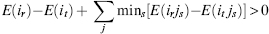
where E(i_r)and E(i_t) are rotamer-template energies, E(i_rj_s) and E(ij_s) are rotamer-rotamer energies for rotamers on residues i and j, and the function minimums selects the rotamer s on residue j that minimizes the argument of the function (Figure 8.4b). According to the original DEE criterion (Figure 8.4a), only when the best energy of a specific rotamer is worse than the worst energy of another rotamer at the same position, it can be eliminated, that is, the minimization part of the above equation is decomposed to a minimization of E(i_rj_s) and maximization of E(t_rj_s), and each rotamer is compared to the rotamers of any protein conformation. As shown in Eq. 8.4, the elimination criterion was relaxed by Goldstein to include rotamers for which other rotamers can be found that have lower energy against an identical conformational background (Goldstein, 1994). In other words, the Goldstein criterion DEE claims that a rotamer can be eliminated if the rotamer’s contribution to the total energy is always reduced by using an alternative rotamer. A conformational background is obtained by fixing each residue in the conformation that most favors the assessed rotamer. A further relaxation of the simple Golstein criterion, termed “general Goldstein criteria” (Figure 8.4c), compares the rotamer to the average of other rotamers taken from the same conformational background (Goldstein, 1994). A rotamer can be eliminated if the average of the other rotamers has a lower energy compared to the assessed rotamer, as then there will always be at least one rotamer that is better. Additional relaxing modifications to the DEE pruning criteria include the use of “split-DEE” (Figure 8.4d). Here, the conformational space is split into partitions within which each of the candidate rotamers can be compared singly (Pierce et al., 2000).

An alternative modification is to use dead-ending pairs (also termed “doubles”) in which a specific combination is dead-ending. In such a case, each one of the rotamers building the pair may not be dead-ending if applied in a different combination. The idea can be generalized into grouping several side chains into super rotamers (Goldstein, 1994; De Maeyer et al., 2000). The super rotamer contains all the possible combinations of the individual side-chain rotamers. While the pruning power of a single rotamer’s interaction with a super rotamer is more intuitive, the implementation of super rotamers is more complex. “Generalized DEE” compares clusters of rotamers instead of individual rotamers and adds a split-DEE scheme for the clusters, thus improving the convergence properties enabling efficient redesign of large proteins (Looger and Hellinga, 2001). The choice of weights to achieve the “average” adds additional complexity. The “enhanced-DEE” algorithm finds these weights via linear programming (Lasters et al., 1995).

The first fully automated design and subsequent experimental validation of a novel sequence for an entire protein utilized the DEE pruning approach (Dahiyat and Mayo, 1997). The fully automated protein design scheme uses a combination of several search methods, each tailored for a different segment of the design scheme (Dahiyat and Mayo, 1996): Following the use of the generalized DEE algorithm, a MC simulation (described later) was executed for the top sequences selected by the DEE. The MC was carried out as the theoretical and actual potential surfaces may be different. In other words, a GMEC selected by the DEE procedure from the theoretical energy landscape may differ from the actual GMEC that is part of the experimental “real” energy landscape. Interestingly, the MC scoring function was derived by comparing structural properties of the designed proteins to experimental stability (melting temperature) in the frame of a quantitative structure-activity relationship (QSAR) (Chapter 34). The QSAR feedback selected polar and nonpolar surface burial parameters, as well as the relative weight of each parameter within the scoring function, thus improving the design algorithm.

Very recently, DEE was used to investigate multistate and flexible structures. The X-DEE (extended-DEE) application searches within discrete subspaces for low-energy states of the protein, for example, the photocycle intermediates of the bacteriorhodopsin light-driven proton pump (Kloppmann et al., 2007). Following the many DEE runs for a large number of subspaces, gap-free lists of low-energy states are generated. Such lists can be utilized for a kinetic study of the transitions between states. To overcome the difficulty of standard DEE in tackling multistate design problems, a type-dependent DEE was recently suggested (Yanover et al., 2007). Standard DEE allows for a rotamer at a certain position to be a potential candidate for elimination by any other rotamer at that position. In contrast, in type-dependent DEE a rotamer may be eliminated based only on comparisons with other rotamers of the same amino acid type. Adding ranges of spatial locations to each rotamer is another approach to intrinsically take into account varying states or natural flexibility. Flexible backbone DEE was applied by adding a constraining box around each residue, thus limiting the measured rotameric interactions by upper and lower bounds. (Georgiev and Donald, 2007). As demonstrated, the pruning power of DEE can be utilized for many cases as long as the rotamer interaction constraints are formulated properly.

Finally, one of the major limitations of DEE is that it does not scale well with the size of the protein. The limitation is especially relevant for large proteins and for the larger structural space that needs to be scanned in protein design. As briefly discussed, one possibility is to hierarchically split a given problem and use the DEE method only for the part of the challenge for which it is optimized.

Self-Consistent Mean Field. SCMF, also known as mean field theory, aims at reducing the cost of combinatorics generated by the interaction terms when summing over all states of a multibody problem. The main idea of the mean field theory is to replace all interactions to any one body with an average or effective interaction. This reduces any multibody problem into an effective one-body problem. Thus, the method is far faster, compared to methods such as DEE, and usually scales polynomially (rather than exponentially) as a function of the size of the assessed variables (e.g., number of residues). Yet, due to the simplified parameterization, SCMF is less accurate and unlike DEE, may fail in finding the optimal solution (Cootes et al., 2000; Voigt et al., 2000). The accuracy is not easy to compare to other methods and depends on the mean field approximation (MFA). The MFA is the minimizing reference system that transforms the multibody interaction to a one-body (zero order) approximation, preferably using noncorrelated degrees of freedom. Thus, SCMF should be applied only in cases where the MFA is valid within the targeted accuracy. In SCMF, the average field, such as energy, is determined self-consistently as the overall cutoff threshold is lowered. SCMF will be demonstrated here via examples that are carefully tailored to fit the MFA and the consistency requirements.

Some of the first applications of SCMF for biological molecules were in the field of protein structure prediction (Section VI in this book). For example, a mean field approach for assigning a unique fold, known as fold recognition (Chapter 31), was applied by Friedrrichs and Wolynes (1989). Finkelstein and Reva (1991) used SCMF to predict β-sandwich structures. While short-range interactions were modeled explicitly, the large number of atoms contributing to the long-range interaction component utilized a mean field approach. Using only the strand directionality (but not strand length) and sequence, their SCMF algorithm identified the folds correctly. As their mean field equation for inter-and intrastrand interactions converged quickly and independently of the starting “field,” this early work concludes that for fold recognition it is the local hydrophobicity that determines the fold.

SCMF was applied for side-chain modeling (Mendes et al., 1999) and expanded to include loop modeling (also known as “gap closure”) (Koehl and Delarue, 1994; Koehl and Delarue, 1995). Loops connecting secondary structures are the least accurate region in homology modeling (Chapter 30) as well as in other protein structure prediction schemes. Consequently, the mean field approach is especially relevant for such modeling. Koehl and Delarue sampled several potential fragments as loop candidates to connect the modeled secondary structures. Each such position requires rotamer library-based modeling of the best side-chain conformation. A similar multicopy approach was used for side-chain modeling. The conformational matrix was weighted according to the relative probabilities of the different backbone fragments. For loop modeling, rather than modeling each fragment discretely, a MFA was built from the conformational matrix and utilized to assess the rotamer-rotamer energies when modeling each side chain sequentially. The iterative procedure was carried out till convergence, confirming the self-consistency of this search method. This loop and side-chain modeling was applied in the 3D-JIGSAW comparative modeling program (Bates et al., 2001). To overcome the lower resolution of the SCMF approach, the online server (http://www.bmm.icnet.uk/servers/3djigsaw) refines the results by trimming the loops for good geometry by adjusting torsion angels as well as adding a short minimization step.

Stochastic Search Methods

Unlike deterministic methods, stochastic methods have a random component and may give a different answer for each run. The “random” character is often given by a random number generator. Notably, it is important to choose a generator that is indeed random, as not all are. One can also test this component to see whether over a large number of runs the scattering is indeed random. For more on commonly used random number generators and pitfalls therein, see Schlick (2002).

Monte Carlo Simulations. MC simulations, a collective name for the usage of an iterative application of random perturbation steps that can be accepted or rejected, has become one of the most common stochastic search procedures. MC is applied in numerous disciplines having a large search space, a large uncertainty of specific parameters, or a combination of both, for example, structural bioinformatics. This simple and efficient technique was largely established in Los Alamos by Metropolis et al. setting the method of generation of trial states along with criteria for accepting or rejecting the MC step (Metropolis et al., 1953). MC can simulate a time-dependent process, such as Brownian dynamics or a static state, such as a rotamer library-based conformational search. For an equilibrium simulation, the probability of residing in a particular state should be that of an equilibrium distribution. As introduced earlier in the chapter in the frame ofergodicity, this implied that the detailed balance criterion must be maintained - a prime concern when setting the MC simulation conditions.

The very name of MC hints at the gambling aspect of this simulation—a random move is attempted using information derived from the latest state. Some criteria for the move are set in advance. These include the amount and type of perturbation applied at each step, namely, the relative segment of the investigated system that undergoes change and the magnitude of the change. More important, in classical MC the direction of the move is random. Next, and most important, the move has to be accepted or rejected. In order to get out of local minima moves that are less favorable should be occasionally accepted. Classic MC applications simulate an equilibrium state that follows a Boltzmann-type distribution—the distribution originally suggested by Metropolis. As such, moves that have a lower minimum will always be accepted, while moves that are less favorable will be accepted with a probability corresponding to the Boltzmann distribution. This simple acceptance criterion not only channels the moves toward the local minima but also allows occasional jumps to bypass local energy barriers, hence exploring other minima. Finally, convergence of the MC application should be addressed. As a stochastic procedure, finding the GMEC is not guaranteed. Consequently, overcoming local minima traps is often approached by applying multiple independent MC runs, each with a predefined number of steps.

Here, MC will be demonstrated for the side-chain conformational search challenge hopefully without losing generality. The conformation ofa protein sequence is composed as a discrete set of residue conformations, that is, α = {α₁,…,α_N}. Such a set can be modeled as a Markov Chain; a discrete-time stochastic process with a Markov property. Having the Markov property means the next state depends solely on the present state and does not directly depend on the other previous states. A single component, for example, α_i, of this Markov Chain MC (often termed MCMC) can be altered. Alternatively, several, or all, of the components can be altered simultaneously. In either case, a new trial rotamer sequence α’ is generated. Following the Metropolis criterion (Metropolis et al., 1953), detailed balance can be achieved by selecting the general form of:

(8.5)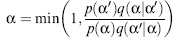

where p(α) is the equilibrium (long time) probability of configuration α, and q(α|α’) is the trial probability associated with generating configuration a’ given that we started with configuration α. The equilibrium probability has the form p(α) ∞ exp(— βF(α))/Z(β), where F(a) is an energy-based scoring function that quantifies how well the sequence matches a particular target structure, and β∞1/T, where T is an effective temperature, and the partition function Z(β) ensures that p(α) is normalized. In classic MC, the trial distribution is independent of the initial distribution, that is, q(α|α’) = q(α’|α). Thus, the equation is reduced to the Metropolis acceptance criteria (Metropolis et al., 1953):

(8.6)

Convergence of the MC protocol can be achieved using a number of methods. For example, a predetermined number of MC steps can be assigned or the simulation can be terminated if a predetermined number of steps does not improve the result. To sample the required landscape comprehensively while focusing on the most probable region in greater detail, a SA scheme may be applied. SA involves a temperature that is initially high allowing for large jumps between local minima and then gradually decreased to carefully investigate the region of interest. The exact cooling rate, which is proportional to the number of MC iterations, is often decided using a trial-and-error procedure in which convergence is assessed on case studies. Notably, the general method of SA can be applied with acceptance probabilities other than the Boltzmann one.

The details of the degree of change between one state (a) and another (a’) depend on the specific MC simulation conducted. In conformational search challenges, changes may include specific residue locations, identities, and rotamers. For example, DeGrado and coworkers applied a SA-MC scheme of 10,000 iterations to design the side chains of transmembrane helices that specifically target natural transmembrane proteins (Yin et al., 2007). Using an exponential cooling schedule, each SA-MC iteration included a single mutation of a protein-protein interface residue. Then, rotamer optimization was applied to the entire ensemble of residues in the helical pair. A further decrease in search size was implemented by including only residues prevalent in transmembrane proteins. The rotamer search space was minimized by including only highly probable rotamers and optimized using the DEE method. Hence, a combination of search and sampling methods was tailored for this protein design task.

OVERCOMING MC LIMITATIONS. MC requires a large number of iterations to achieve convergence as it is challenged by the large phase space to be explored as well as by the roughness of the energy landscape. Thus, one of the main challenges in MC simulations is how to focus the search, namely, minimize the sampled space to the minimum required for convergence. While SA will change the probability to accept a less favorable trial as the simulation proceeds, it will still give each trial configuration an equal likelihood, that is, q(a|a’) = q(a’|a). Changing this relationship may enable a biased search toward areas of increased likelihood, hopefully without missing regions bordered by high-energy barriers. Indeed, to avoid local minima traps a very slow cooling rate is often required. Next, we will briefly present examples of MC modifications to overcome these limitations including MC-quench, biased MC, SCMF-MC, and replica exchange-biased MC.

A MC-quench procedure recognizes that each trial configuration had an equal likelihood and was assessed sequentially. In other words, each position is not optimized to the final structure but to a trial predecessor of this structure.Consequently, when the end result is achieved, there may be specific locations that may be further improved as their environment has changed after they were assessed. Assessing side-chain position, Mayo and coworkers found that by taking the resulting structure from an MC-SA procedure and minimizing the energy of all possible rotamers of each location the solution is improved dramatically (Voigt et al., 2000).

A biased MC procedure can focus the simulation toward more probable attempted trials. Similar to accepting less preferred moves in classical MC, biased MC will not throw away moves toward less preferred regions but rather provide such moves with a lower probability. Thus, the stochastic movement is guided by the local energy facilitating large movements and increased acceptance rates. Mathematically, we have

(8.7)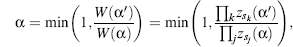

where W, the Rosenbluth weight (Rosenbluth and Rosenbluth, 1955), can be defined as the relative portion of available sites multiplied by the weight of the previous state. This can be described by

(8.8)

Such an approach requires a computational overhead in the need to calculate the relative probabilities in each biased MC step. This overhead should be weighted against the added efficiency resulting from the biasing. Therefore, the cost-effectiveness of biased MC is best valued in specific applications. For example, growing a molecule toward acceptable structures is often done via the configurational-biased MC method (Siepmann, 1990). McCammon and coworkers recently applied the method for the continuous exploration of side-chain placement (Jain et al., 2006). This interesting application combines a molecular mechanics potential function with a rotamer library that can be extended around the discrete rotamers. Such fine-tuning of flexibility is especially important in the most interesting areas of the protein, namely, functional sites and protein-protein interfaces. Notably, for specific cases a very efficient end-transfer configurational-biased MC can be applied, for example, deleting one end of a polymer and growing it on the other side (Arya and Schlick, 2007). Such a technique is best suited for sampling linear combinations of biopolymers such as nucleic acids (Chapter 3) as applied by Arya and Schlick, in combination with other MC methods, to study chromatic folding (Arya and Schlick, 2006).

Biased MC was applied, for example, in an early attempt at homology modeling. Holm and Sander (1992) attempted to bias the rotamer weights used for side-chain optimization. Statistics on rotamer searches in the optimized configurations from a large number of short MC runs were collected and the new “learned” rotamer frequencies were applied to bias new moves toward high-probability regions. Baker and coworkers applied the RosettaDesign algorithm (itself an extension of their ab initio structure prediction algorithm—see Chapter 32) in an on-the-fly biased-MC way (Dantas et al., 2003). Here, the first MC runs tested all possible 20 residues for each position in the designed protein. The list of acceptable mutations was utilized to bias a second MC procedure enabling the sampling of a much larger rotamer library, thus refining the results. In the same line of thought, one can conduct MC procedures iteratively with each iteration hierarchically focusing on a different search space, for example, cycling between side-chain design and backbone optimization (Kuhlman et al., 2003).

Synthesizing the sampling power of MC and the speed of SCMF methods, Zou and Saven (2003) offered a SCMF-biased MC method for designing and sampling protein sequences. Following a SCMF approach (described earlier in the chapter), the sequence identity probabilities for each location were precalculated prior to the MC sampling. These weights are utilized to bias the MC sampling resulting in efficient sampling of low-energy sequences and enabling fast SA cooling rates. Following the above general equation, as q(α|α’)/q(α’|α) = p(α)/p(α’), the acceptance probability is reduced to

(8.9)

An alternative approach to more efficient scanning of the target landscape focuses on the temperature protocol applied to the simulation, that is, protocols other than SA. For example, the low-temperature simulation may periodically be allowed to jump (jump walking or J-walking) to a high-temperature simulation (Frantz et al., 1990). A variation of J-walking is the replica exchange method (REM) (Geyer and Thompson, 1995). In this method, noninteracting copies (replicas) of the original system at different temperatures are simulated independently and simultaneously. Pairs of replicas are exchanged with a specific transition probability that maintains each temperature’s equilibrium ensemble distribution, thus realizing a random walk in energy space and facilitating the passage over energy barriers. Such a method is most suitable for sampling the conformation of a rough energy landscape, as shown for a pentapeptide conformation search (Hansmann, 1997). Yang and Saven applied REM-MC and REM-biased MC to redesign the calcium binding protein calbindin (Yang and Saven, 2005). The output energy, the redesigned sequence, was lowest when applying REM-biased MC compared to REM-MC that in turn was lower relative to SA-MC. Possibly even more important, an analysis of specific pivotal residues showed that the REM-biased MC method overcome local minima traps showing an improved sampling of the low-energy sequences.

In conclusion, despite the two limiting aspects of MC, large sampling space and lack of guarantee to convergence, MC became widely used due to a high success rate and many incorporated tricks applied to overcome limitations. There is no one answer to the best way to tailor an MC approach to a specific problem. Unfortunately, there have been few benchmarks that objectively compare sampling methods, let alone MC variations. The success of MC and other stochastic methods is not only due to our understanding of the investigated search problems and the availability of fast computers, but also due to the fact that most often multiple answers can satisfy the investigated question. Finally, there continues to be a wide variety of MC variations, and the above examples are only used to introduce this powerful method.

Stochastic Population Search and Sampling Methods. Most search and sampling methods focus on finding a single best solution. However, often it would be beneficial to aim at finding a (relatively) small top-scoring population that can be either further assessed by higher resolution methods or fully checked experimentally. One option to achieve such a scheme is by hierarchically combining methods of increasing resolution. Thus, every method does not necessarily provide a population but a representative solution of smaller subpopulations that are subject to further higher resolution search and sampling. Examples include side-chain and main-chain modeling, where each part of the problem should be addressed in a different resolution (Kuhlman et al., 2003; Yin et al., 2007). In other cases, for example, energy minimization, a protocol of different minimization methods with growing resolution results is hierarchically devised, for example, grid search, followed by conjugated gradient and adapted basis Newton Raphson (Chapter 37).

A hierarchical population approach may be devised by deterministic approaches that do not converge but do result in a manageable top-scoring population. For example, in interesting work by Singh and coworkers on side-chain positioning, integer linear programming was combined with simple DEE to reduce search space (Kingsford et al., 2005). In brief, linear programming aims to minimize a linear equation subject to constraints. In this specific case, this is the energy function of rotamers subject to choosing a single rotamer per residue and calculating interresidue contact energy only for the chosen rotamers. By relaxing the integrality of the latter constraint to include only rotamers that interact, the algorithm is reduced to a much faster polynomial-time linear programming heuristic. However, this heuristic will not find the GMEC requiring full integer linear programming in some cases. In such cases, DEE is applied first to prune the search space considerably. Next, the solutions not pruned by DEE are subject to the integer linear programming. Despite the fact that the DEE pruning mechanism is not tailored to find the optimal subpopulation of solutions, this application yields high-accuracy results similar to those obtained by far less efficient algorithms. In this example, DEE is specifically targeted not to find the GMEC but to enable a manageable data set for an algorithm that could not run practically on the full data set. In this context, it should be noted that others have also combined the power of DEE with complementary search techniques to produces low-energy populations. For example, Leach and Lemon (1998) combined DEE with the A* algorithm that finds the “least cost” path of a graph. With the added computational cost, they assess the side-chain contribution to the conformational entropy of the folded protein.

Iterative Stochastic Elimination (ISE), developed by the Goldblum group, aims at producing a manageable ensemble of a best population that can be further searched by more detailed or even exhaustive search methods (Glick et al., 2002). Rather than focusing on finding one GMEC solution, this algorithm puts emphasis on forming a high-scoring ensemble. After a quick elimination of backbone clashing rotamers and side-chain to side-chain clashing rotamer pairs, the algorithm introduces an interesting stochastic stage. Following sampling at random of a large population of conformations, a distribution function of the energies in all sampled conformations is constructed. Then, the rotamers of the best and worst results are compared. The stochastic stage is repeated with every cycle excluding rotamers that were present in the set of the worst results but not in the set of best results of the previous iteration. The method was applied successfully on a number of other search challenges, for example, predicting the conformation of protein-protein interfaces using data from structures in the unbound state (Noy et al., 2007).

“Biological” approaches such as GA or NN have been applied to a number of search and sampling challenges in structural bioinformatics. For example, GA was utilized for protein structure prediction (Pedersen and Moult, 1996) and protein design (Jones, 1994). Briefly, the investigated degrees of freedom, for example, translational, rotational, and internal degrees of freedom, are encoded into “genes” that are represented by the real values of these degrees of freedom. Mutations at a fixed rate, often corresponding to an average of one mutation per sequence, are applied to a population of random sequences. A scoring function, such as energy, is calculated for each mutant. The best scoring mutant sequences are kept as well as subjected to crossovers among themselves. These “most fit” surviving sequences, namely, the new generation, is subjected again to a cycle of mutations and crossovers. The cycles are fixed to a certain number or until the energy of the new generations does not improve. The basic algorithm has many additional possible modifications, for example, a migration operator responsible for moving individual sequences from one subpopulation to another. In the case of conformational searching, the genes are usually a subset of coordinates with a potential energy defining the fitness.

The population dynamics of GAs makes larger moves than the typical MC, and thus can sample a large space rapidly overcoming local energy barriers. While the overall number of required steps is usually small, the generation of each GA cycle is more costly than other methods. In addition, while keeping only the top-scoring members of the population, the nature of this error-embedded and inbred population may result in slower, and sometimes lack of, convergence. This is especially true of highly coupled systems and cases where the coupling is not adjacent in location, for example, structural interactions of locations that are not close in sequence. Mayo and coworkers compared the GA to other protein design algorithms (Voigt et al., 2000). They found that GA performs better than the often locally trapped MC and SCMF methods in spite of the possible intrinsic convergence problems. Yet, the simple fine-tuning of MC to MC-quench (section ’’Overcoming MC limitations ) outperformed GA in the tested examples. Brooks and coworkers compared MD-SA, GA, and MC as search procedures for flexible docking (Vieth et al., 1998). All three methods showed overall similar efficiency with GA scoring the best when searching a small space but not for the larger space, where MD-SA was the best.

A neural network, another method to extract patterns embedded in high-dimensional data, is often applied in conjunction with other methods. Hwang and Liao (1995) applied NN along with a MC-SA scheme for side-chain modeling. Kono and Doi (1994) applied a NN algorithm to design protein cores using a reduced set of residue types. Schneider et al. applied NN for peptide design by processing QSAR information from an experimental training set of peptides and computationally designed low-energy scoring antagonist peptides against the β₁-adenoreceptor (Schneider et al., 1998).

Probabilistic approaches to protein design are complementary to those that search for particular sequences via optimization of a scoring function (Kono and Saven, 2001; Saven, 2002; Fu et al., 2003; Park et al., 2005). Such methods estimate the site-specific probabilities of the amino acids within sequences that are structurally consistent with a target structure. These structural interactions are quantified by atomistic energy functions that address rotamer-backbone, rotamer-rotamer, and rotamer-solvent interactions. In addition, a variety of constraints may be introduced to specify function, such as the placement of side-chain ligands to form a metal binding site. The site-specific amino acid probabilities are determined by maximizing an effective entropy function subject to constraints on the sequences. The method has been extended so as to bias SA methods (Zou and Saven, 2003) and include symmetric quaternary structures (Fu et al., 2003). Such a statistical computationally assisted design strategy (SCADS) has been applied to design a variety of proteins, including water-soluble analogues of the membrane spanning potassium channel KcsA (Slovic et al., 2004).

Other Methods to Search the Complex Phase Space—Random Walk, Umbrella Sampling, and Replica Exchange. Local minima within a phase space, such as an energy landscape, pose a challenge to detailed searching of the space. Sampling such a surface must specifically look for the small but potentially deep wells distributed along the rough energy landscape. Several designated methods for better sampling of a complex structural space have been developed in the context of molecular dynamics. Consequently, complementary additional sampling topics will be discussed in Chapter 37. For an example of replica exchange sampling, see section “Overcoming MC Limitations.”

DATA ANALYSIS AND REDUCTION

A topic intimately connected to the search and sampling challenge is the way data are analyzed and reduced. While this requires a chapter of its own, some basic terms are briefly introduced here. Also, some topics in this field that are common in the study of protein motion (Chapter 37) are discussed therein. Notably, the search and sampling strategy should be targeted to the available data analysis methods, which in turn may provide results requiring further search and sampling of the target space.

Similarity measures, for example, via support vector machines (SVM) and designated cluster and pattern analysis, for example, principal component analysis (PCA) and normal mode analysis (NMA) are powerful tools to decipher high-dimensionality data. NMA is rapidly developing into bringing quick biophysical insight that was not long ago not in reach—readers are referred to the excellent recent text-book on NMA theory and applications edited by Cui and Bahar (2006) and to Chapter 37. PCA can be viewed as a generalizing extension of the NMA concept (Cui and Bahar, 2006). PCA aims to reduce the dimensionality of a data set consisting of a large number of interrelated variables, while retaining as much as possible of the variation present in the data set. This reduction is achieved by transforming to a new set of variables, the principal components, which are uncorrelated and ordered so that the first few retain most of the variation present in all the original variables (Jolliffe, 2002). PCA involves calculation of the eigenvalue decomposition of a data covariance matrix or can utilize singular value decomposition (SVD) of the data matrix. SVD is a factorization of rectangular matrices, that is, a generalization of the eigenvalue decomposition for square matrices. The SVD approach is more efficient compared to the classic principal component calculation, as formulation of the covariance matrix is not required. Beyond the straightforward use in protein motion (Chapter 37), for example, as shown by Ichiye and Karplus (1991), this general method can be utilized to compare complex data such as protein structures (Zhou et al., 2006) or NMR spectra (Ross and Senn, 2003).

SVM is a machine learning approach for classifying data (Noble, 2006). Briefly, a classifying hyperplane between groups of objects is defined using a known training set. The hyperplane is constructed so that it will optimize a “maximum margin,” namely, a maximum distance from each of the objects within the groups it separates. It is built using a kernel function of higher dimensionality compared to the original data. Notably, the dimensionality must not be too high to avoid overfitting as well as increased complexity. Finally, accounting for the intrinsic noise of the data, a soft margin, extending from the hyperplane to the nearest object in each group, is assigned. The high prediction power of SVM and suitability to the intrinsic nature of structural bioinformatics data resulted in growing popularity of this method. Just to name some examples, recently SVMs were used to predict (1) functionally flexible regions from primary sequence (Gu et al., 2006), (2) protein binding sites using sequence and structure homolog information (Chung et al., 2006), (3) protein folding kinetic order and rate using kinetic and mechanistic information from known structure (Capriotti and Casadio, 2007), (4) folds within multidomain protein structures (Redfern et al., 2007), (5) membrane binding proteins from primary sequence using information from known such structures (Bhardwaj et al., 2006), and (6) local ordered regions within the “random coil” secondary structure region using sequence information (Zimmermann and Hansmann, 2006).

CONCLUDING REMARKS

In this introductory chapter, a glimpse into the vast topic of search and sampling in structural bioinformatics is provided. As evident in the many references to other chapters in this book, search and sampling methods are pivotal in most applications of structural bioinformatics research. As a broad and evolving field, many search and sampling methods and specific applications were not included. With increasing computational power, the use of search and sampling methods producing the single solution or low-energy populations of the requested target is expected to increase. Beyond the possibility of using more detailed computational methods to further assess such a population, high-throughput experimental techniques can also be applied to such a manageable set of candidate results. However, despite the growing computer power, many questions now and into the future in structural bioinformatics lie in an expanding space far too large to exhaustively scan, so search and sampling techniques will continue to be critical.

Contrary to the success stories described here, some structural bioinformatics results are incorrect as a result of the lack of sufficient understanding of limitations and errors within the different search and sampling methods. Thus, even more important than understanding the success of each method is fully recognizing the limitations and optimal resolution achieved by each one of these methods. We hope this chapter is a step in this direction.

ACKNOWLEDGMENTS

Thanks to Jason E. Donald, RolandL. Dunbrack, Scott Shandler, Joanna S. Slusky, and Cinque Soto for critical reading of the manuscript. IS was funded by the European Molecular Biology Organization (EMBO) and by the Human Frontier Science Program Organization (HFSPO).

REFERENCES (Including Remarks on Recommended Further Reading)

Arya G, Schlick T (2006): Role of histone tails in chromatin folding revealed by a mesoscopic oligo- nucleosome model. Proc Natl Acad Sci USA 103(44):16236-16241.

Arya G, Schlick T (2007): Efficient global biopolymer sampling with end-transfer configurational bias

Monte Carlo. JChemPhys 126(4):044107. Baldi P, Brunak S (2001): Bioinformatics: The Machine Learning Approach. MIT Press. Bates PA, Kelley LA, MacCallum RM, Sternberg MJ (2001): Enhancement of protein modeling by human intervention in applying the automatic programs 3D-JIGSAW and 3D-PSSM. Proteins (Suppl. 5): 39-46.

Bayes T (1763): An essay towards solving aproblemin the doctrine ofchances. PhilosTransRoySoc 53:370.

Becker OM(2001): Conformationalanalysis. In: Becker OM, MacKerell AD, Roux B, Watanabe M, editors. Computational Biochemistry and Biophysics. Marcel Dekker, pp 69-90.

Becker OM, MacKerell AD, et al. , editors (2001): Computational Biochemistry and Biophysics. New York: Marcel Dekker, Inc. [An excellent text on computational biochemistry and biophysics that is focused largely on molecular motion. The book includes several important introductory chapters along with advanced applications.B.

ecker OM, Shacham S, et al. (2003): Modeling the 3D structure of GPCRs: advances and application to drug discovery. Curr Opin Drug Discov Devel 6(3):353-361.

Berman HM, Battistuz T, et al. (2002): The Protein Data Bank. Acta Crystallogr D Biol Crystallogr 58 (Pt 6 No 1):899-907.

Bhardwaj N, Stahelin RV, et al. (2006): Structural bioinformatics prediction of membrane-binding proteins. J Mol Biol 359(2):486-495.

Bradley LH, Wei Y, et al. (2007): Protein design by binary patterning of polar and nonpolar amino acids. Methods Mol Biol 352:155-166.

Brenner SE, Koehl P, et al. (2000): The ASTRAL compendium for protein structure and sequence analysis. Nucleic Acids Res 28(1):254-256.

Camacho CJ (2005): Modeling side-chains using molecular dynamics improve recognition of binding region in CAPRI targets. Proteins 60(2):245-251.

Capriotti E, Casadio R (2007): K-Fold: a tool for the prediction of the protein folding kinetic order and rate. Bioinformatics 23(3):385-386.

Chung JL, Wang W, et al. (2006): Exploiting sequence and structure homologs to identify protein-protein binding sites. Proteins 62(3):630-640.

Cootes AP, Curmi PM, et al. (2000): Automated protein design and sequence optimisation: scoring functions and the search problem. Curr Protein Pept Sci 1(3):255-271.

Cui Q, Bahar I, editors. (2006): Normal Mode Analysis: Theory and Applications to Biological and Chemical Systems. Mathematical and Computational Biology Series. Chapman & Hall/CRC. [A new and highly recommended book on theory and applications of normal mode analysis. The book is complementary to the book edited by Becker et al., (2001) and presents the theory behind NMA as well as applications such as structural refinement, large motions, conformational sampling, and diffusion in liquids.]

Dahiyat BI, Mayo SL (1996): Protein design automation. Protein Sci 5(5):895-903.

Dahiyat BI, Mayo SL (1997): De novo protein design: fully automated sequence selection. Science 278(5335):82-87.

Dantas G, Kuhlman B, et al. (2003): A large scale test of computational protein design: folding and stability of nine completely redesigned globular proteins. J Mol Biol 332(2):449-460.

De Maeyer M, Desmet J, et al. (1997): All in one: a highly detailed rotamer library improves both accuracy and speed in the modelling of side chains by dead-end elimination. Fold Des 2 (1):53-66.

De Maeyer M, Desmet J, et al. (2000): The dead-end elimination theorem: mathematical aspects, implementation, optimizations, evaluation, and performance. Methods Mol Biol 143:265-304.

Deshpande N, Addess KJ, et al. (2005): The RCSB Protein Data Bank: a redesigned query system and relational database based on the mmCIF schema. Nucleic Acids Res 33(Database issue): D233-D237.

Desmet J, Demaeyer M, et al. (1992): The dead-end elimination theorem and its use in protein side- chain positioning. Nature 356(6369):539-542.

Dunbrack RL Jr, Karplus M (1994): Conformational analysis of the backbone-dependent rotamer preferences of protein side chains. Nat Struct Biol 1(5):334-340.

Dunbrack RL Jr, Cohen FE (1997): Bayesian statistical analysis of protein side-chain rotamer preferences. Protein Sci 6(8):1661-1681.

Dunbrack RL Jr (2001): Bayesian statistics in molecular and structural biology. Computational Biochemistry And Biophysics. In: Becker OM, MacKerell AD, Roux B, Watanabe M,editors. New York: Marcel Dekker, p. 512.

Dunbrack RL Jr (2002): Rotamer libraries in the 21st century. Curr Opin Struct Biol 12(4):431-440.

Dwyer MA, Looger LL, et al. (2004): Computational design of a biologically active enzyme. Science 304(5679):1967-1971.

Eyal E, Najmanovich R, et al. (2004): Importance of solvent accessibility and contact surfaces in modeling side-chain conformations in proteins. J Comput Chem 25(5):712-724.

Finkelstein AV, Reva BA (1991): A search for the most stable folds of protein chains. Nature 351(6326):497-499.

Fischer D, Tsai CJ, et al. (1995): A 3D sequence-independent representation of the protein data bank. Protein Eng 8(10):981-997.

Frantz DD, Freeman DL, et al. (1990): Reducing quasi-ergodic behavior in Monte Carlo simulations by J-walking—applications to atomic clusters. J Chem Phys 93(4):2769-2784.

Friedberg I, Godzik A (2007): Functional differentiation of proteins: implications for structural genomics. Structure 15(4):405-H5.

Friedrichs MS, Wolynes PG (1989): Toward protein tertiary structure recognition by means of associative memory Hamiltonians. Science 246(4928):371-373.

Fu X, Kono H, et al. (2003): Probabilistic approach to the design of symmetric protein quaternary structures. Protein Eng 16(12):971-977.

Georgiev I, Donald BR (2007): Dead-end elimination with backbone flexibility. Bioinformatics 23 (13):i185-i194.

Geyer CJ, Thompson EA (1995): Annealing Markov-Chain Monte-Carlo with applications to ancestral inference. J Am Stat Assoc 90(431):909-920.

Gilks WR, Richardson S et al., editors (1996): Markov Chain Monte Carlo in Practice. Chapman & Hall/CRC.

Glick M, Rayan A, et al. (2002): A stochastic algorithm for global optimization and for best populations: a test case of side chains in proteins. Proc Natl Acad Sci USA 99(2):703-708.

Goldstein RF, (1994): Efficient rotamer elimination applied to protein side-chains and related spin glasses. Biophys J 66(5):1335-1340.

Goodman CM, Choi S, et al. (2007): Foldamers as versatile frameworks for the design and evolution of function. Nat Chem Biol 3(5):252-262.

Greene LH, Lewis TE, et al. (2007): The CATH domain structure database: new protocols and classification levels give a more comprehensive resource for exploring evolution. Nucleic Acids Res 35(Database issue):D291-D297.

Gu J, Gribskov M, et al. (2006): Wiggle-predicting functionally flexible regions from primary sequence. PLoS Comput Biol 2(7):e90.

Halperin I, Ma B, et al. (2002): Principles of docking: an overview of search algorithms and a guide to scoring functions. Proteins 47(4):409-443.

Hamelberg D, Mongan J, et al. (2004): Accelerated molecular dynamics: a promising and efficient simulation method for biomolecules. J Chem Phys 120(24):11919-11929.

Hansmann UHE (1997): Parallel tempering algorithm for conformational studies of biological molecules. Chem Phys Lett 281(1-3):140-150.

Herzyk P, Hubbard RE (1993): A reduced representation of proteins for use in restraint satisfaction calculations. Proteins 17(3):310-324.

Hobohm U, Scharf M, et al. (1992): Selection of representative protein data sets. Protein Sci 1(3):409-417.

Hobohm U, Sander C (1994): Enlarged representative set of protein structures. Protein Sci 3(3):522-524.

Holm L, Sander C (1992): Fast and simple Monte Carlo algorithm for side chain optimization in proteins: application to model building by homology. Proteins 14(2):213-223.

Holm L, Sander C (1996): Mapping the protein universe. Science 273(5275):595-603.

Hou J, Sims GE, et al. (2003): A global representation of the protein fold space. Proc Natl Acad Sci USA 100(5):2386-2390.

Hwang JK, Liao WF (1995): Side-chain prediction by neural networks and simulated annealing optimization. Protein Eng 8(4):363-370.

Ichiye T, Karplus M (1991): Collective motions in proteins: a covariance analysis of atomic fluctuations in molecular dynamics and normal mode simulations. Proteins 11(3):205-217.

Jain T, Cerutti DS, et al. (2006): Configurational-bias sampling technique for predicting side-chain conformations in proteins. Protein Sci 15(9):2029-2039.

Jiang L, Kuhlman B, et al. (2005): A “solvated rotamer” approach to modeling water-mediated hydrogen bonds at protein-protein interfaces. Proteins 58(4):893-904.

Jolliffe IT, (2002): Principal Component Analysis. Springer.

Jones DT (1994): De novo protein design using pairwise potentials and a genetic algorithm. Protein Sci 3(4):567-574.

Kamtekar S, Schiffer JM, et al. (1993): Protein design by binary patterning of polar and nonpolar amino acids. Science 262(5140):1680-1685.

Kang SG, Saven JG (2007): Computational protein design: structure, function and combinatorial diversity. Curr Opin Chem Biol 11(3):329-334.

Kingsford CL, Chazelle B, etal. (2005): Solving and analyzing side-chain positioning problems using linear and integer programming. Bioinformatics 21(7):1028-1036.

Kloppmann E, Ullmann GM, et al. (2007): An extended dead-end elimination algorithm to determine gap-free lists of low energy states. J Comput Chem 28(14):2325-2335.

Koehl P, Delarue M (1994): Application of a self-consistent mean field theory to predict protein side-chains conformation and estimate their conformational entropy. J Mol Biol 239(2):249-275.

Koehl P, Delarue M (1995): A self consistent mean field approach to simultaneous gap closure and side-chain positioning in homology modelling. Nat Struct Biol 2(2):163-170.

Kono H, Doi J (1994): Energy minimization method using automata network for sequence and side- chain conformation prediction from given backbone geometry. Proteins 19(3):244-255.

Kono H, Saven JG (2001): Statistical theory for protein combinatorial libraries. Packing interactions, backbone flexibility, and the sequence variability of a main-chain structure. J Mol Biol 306(3):607-628.

Kuhlman B, Dantas G, et al. (2003): Design of a novel globular protein fold with atomic-level accuracy. Science 302(5649):1364-1368.

Kussell EL, Shakhnovich EI (1999): Analytical approach to the protein design problem. Phys Rev Lett 83(21):4437-4440.

Lassila JK, Privett HK, et al. (2006): Combinatorial methods for small-molecule placement in computational enzyme design. Proc Natl Acad Sci USA 103(45):16710-16715.

Lasters I, De Maeyer M, et al. (1995): Enhanced dead-end elimination in the search for the global minimum energy conformation of a collection of protein side chains. Protein Eng 8(8):815-822.

Leach AR, Lemon AP (1998): Exploring the conformational space of protein side chains using deadend elimination and the A* algorithm. Proteins 33(2):227-239.

Leach AR (2001): Molecular Modeling: Principles and Applications. Prentice Hall. [A practical guide to macromolecular modeling. This 2nd edition goes deep into the scientific and the practical challenges facing molecular modelers.]

Levinthal C (1969): How to fold graciously. In: DeBrunner P, Tsibris J, Munck E. Mossbauer Spectroscopy in Biological Systems. Proceedings of a Meeting Held at Allerton House, Monticello, IL. Urbana, IL: University of Illinois Press, pp 22-24.

Levitt M (1976): A simplified representation of protein conformations for rapid simulation of protein folding. J Mol Biol 104(1):59-107.

Liu JS (2001): Monte Carlo Strategies in Scientific Computing. Springer.

Looger LL, Hellinga HW (2001): Generalized dead-end elimination algorithms make large-scale protein side-chain structure prediction tractable: implications for protein design and structural genomics. J Mol Biol 307(1):429-445.

Looger LL, Dwyer MA, etal. (2003): Computational design of receptor and sensor proteins with novel functions. Nature 423(6936):185-190.

Lovell SC, Word JM, et al. (2000): The penultimate rotamer library. Proteins 40(3):389-408.

MacKay DJC, (2005): Information Theory, Inference and Learning Algorithms. Cambridge: Cambridge University Press. Mendes J, Baptista AM, et al. (1999): Improved modeling of side-chains in proteins with rotamer- based methods: a flexible rotamer model. Proteins 37(4):530-543.

Mendes J, Soares CM, et al. (1999): Improvement of side-chain modeling in proteins with the self-consistent mean field theory method based on an analysis of the factors influencing prediction. Biopolymers 50(2):111-131.

Metropolis N, Rosenbluth AW, et al. (1953): Equation of state calculations by fast computing machines. J Chem Phys 21(6):1087-1092.

Murzin AG, Brenner SE, et al. (1995): SCOP: a structural classification of proteins database for the investigation of sequences and structures. J Mol Biol 247(4):536-540.

Neumann JV (1932): Proof of the Quasi-Ergodic Hypothesis. Proc Natl Acad Sci USA 18(1):70-82.

Noble WS (2006): What is a support vector machine? Nat Biotechnol 24(12):1565-1567.

Noy E, Tabakman T, et al. (2007): Constructing ensembles of flexible fragments in native proteins by iterative stochastic elimination is relevant to protein-protein interfaces. Proteins 68(3):702-711.

Nussinov R, Wolfson HJ (1991): Efficient detection of three-dimensional structural motifs in biological macromolecules by computer vision techniques. Proc Natl Acad Sci USA 88(23): 10495-10499.

Park S, Kono H, et al. (2005): Progress in the development and application of computational methods for probabilistic protein design. Comp Chem Eng, 29:407-421.

Park S, Yang X, et al. (2004): Advances in computational protein design. Curr Opin Struct Biol 14(4):487-494.

Pedersen JT, Moult J (1996): Genetic algorithms for protein structure prediction. Curr Opin Struct Biol 6(2):227-231.

Peterson RW, Dutton PL, et al. (2004): Improved side-chain prediction accuracy using an ab initio potential energy function and a very large rotamer library. Protein Sci 13(3):735-751.

Pierce NA, Spriet JA, et al. (2000): Conformational splitting: a more powerful criterion for dead-ending elimination. J Comput Chem 21(11):999-1009.

Ponder JW, Richards FM (1987): Internal packing and protein structural classes. Cold Spring Harb Symp Quant Biol 52:421-428.

Redfern OC, Harrison A, et al. (2007): CATHEDRAL: a fast and effective algorithm to predict folds and domain boundaries from multidomain protein structures. PLoS Comput Biol 3(11):e232.

Rosenberg M, Goldblum A(2006): Computational protein design: anovelpathtofutureproteindrugs. Curr Pharm Des 12(31):3973-3997.

Rosenbluth MN, Rosenbluth AW (1955): Monte-Carlo calculation of the average extension of molecular chains. J Chem Phys 23(2):356-359.

Ross A, Senn H (2003): Automation of biomolecular NMR screening. Curr Top Med Chem 3(1):55-67.

Saven JG (2001): Designing protein energy landscapes. Chem Rev 101(10):3113-3130.

Saven JG (2002): Combinatorial protein design. Curr Opin Struct Biol 12(4):453-458.

Schlick T (2002): Molecular Modeling and Simulation: An Interdisciplinary Guide. Springer [A comprehensive guide on molecular modeling and simulation. The book is aimed for newcomers and novices alike. It assumes little background yet focuses on the mathematical formulation.]

Schneider G, Schrodl W, et al. (1998): Peptide design by artificial neural networks and computer-based evolutionary search. Proc Natl Acad Sci USA 95(21):12179-12184.

Shapovalov MV, Dunbrack RL Jr (2007): Statistical and conformational analysis of the electron density of protein side chains. Proteins 66(2):279-303.

Shetty RP, De Bakker PI, et al. (2003): Advantages of fine-grained side chain conformer libraries. Protein Eng 16(12):963-969.

Shlyk-Kerner O, Samish I, et al. (2006): Protein flexibility acclimatizes photosynthetic energy conversion to the ambient temperature. Nature 442(7104):827-830.

Siepmann JI (1990): A method for the direct calculation of chemical potentials for dense chain systems. Mol Phys 70(6):1145-1158.

Simons KT, Kooperberg C, et al. (1997): Assembly of protein tertiary structures from fragments with similarlocal sequences using simulated annealing and Bayesian scoring functions. JMolBiol 268(1):209-225.

Slovic AM, Kono H, et al. (2004): Computational design of water-soluble analogues of the potassium channel KcsA. Proc Natl Acad Sci USA 101(7):1828-1833.

Szasz D (1994): Boltzmann’s Ergodic Hypothesis, a Conjecture for Centuries? Presented at International symposium in honor of Boltzmann’s 150th birthday, Vienna.

Thiruv B, Quon G, et al. (2005): Nh3D: a reference dataset of non-homologous protein structures. BMC Struct Biol 5:12.

Vieth M, Hirst JD, etal. (1998): Assessing search strategies for flexible docking. J Comput Chem 19 (14):1623-1631.

Voigt CA, Gordon DB, et al. (2000): Trading accuracy for speed: a quantitative comparison of search algorithms in protein sequence design. J Mol Biol 299(3):789-803.

Wang G, Dunbrack RL Jr (2005): PISCES: recent improvements to a PDB sequence culling server. Nucleic Acids Res 33(Web Server issue):W94-W98.

Xiang Z, Honig B (2001): Extending the accuracy limits of prediction for side-chain conformations. J Mol Biol 311(2):421-130.

Yang X, Saven JG (2005): Computational methods for protein design and protein sequence variability: biased Monte Carlo and replica exchange. Chem Phys Lett 401(1-3):205-210.

Yanover C, Fromer M, et al. (2007): Dead-end elimination for multistate protein design. J Comput Chem 28(13):2122-2129.

Yin H, Slusky JS, et al. (2007): Computational design of peptides that target transmembrane helices. Science 315(5820):1817-1822.

Zhou X, Chou J, et al. (2006): Protein structure similarity from principle component correlation analysis. BMC Bioinformatics 7:40.

Zimmermann O, Hansmann UH (2006): Support vector machines for prediction of dihedral angle regions. Bioinformatics 22(24):3009-3015.

Zou JM, Saven JG (2003): Using self-consistent fields to bias Monte Carlo methods with applications to designing and sampling protein sequences. J Chem Phys 118(8):3843-3854.