9

MOLECULAR VISUALIZATION

Steven Bottomley and Erik Helmerhorst

INTRODUCTION

Visual images are powerful. Images can turn something that may be unseen, abstract, theoretical, or complex into something real and purposeful. Visual images are not just decorations. In a glance, they can add meaning to a message, help people learn, and provide insight that is not possible by looking at the raw data alone. Scientific visualization generates visual images from data generated by scientific experiment and theory. It aims to discover new knowledge by distilling mountains of data into something immediately useful. Traditionally, line graphs, two-dimensional (2D) plots, three-dimensional (3D) plots, mathematical models, physical models, specimens, photographs, drawings, movies, and symbols are used to visualize scientific data. The computer has now become a convenient, and powerful, tool not only for traditional scientific visualization, but also for more challenging visualization tasks involving computer graphics, animations, modeling, and simulations. The importance of computer visualization to science is showcased in annual ’Visualization Challenge’ competitions (Nesbit and Bradford, 2006) and IEEE Visualization Conferences (Table 9.1).

Molecular Visualization

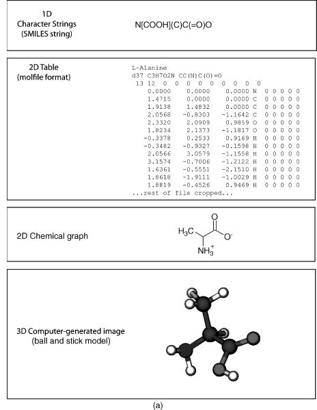
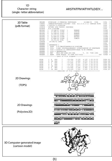
Molecular visualization is a way of seeing the abstract and unseen atomic and molecular world. It uses graphics to study structure, properties, and functions of molecules (Breithaupt, 2006). Consequently, it is also called molecular graphics (Henkel and Clarke, 1985). Small molecules (Figure 9.1a) and macromolecules (Figure 9.1b) can be represented in various ways such as a formula or character format in one dimension (1D), 2D drawings, 2D tables, 3D physical models, or 3D computer-generated models. The SMILES string format (Weininger, 1988) is useful for representing atom connectivity and bond order of small molecules, but awkward for representing macromolecules. Consequently, the primary structure of protein, DNA, and RNA is commonly represented by their one-letter codes. The peptide bond between residues of proteins, or the phosphodiester bond between nucleotides in DNA and RNA, is implicit in the 1D strings. Recently, the primary structure of DNA has also been represented as a 2D graph (Dai, Liu, and Wang, 2006). Character strings, using standard abbreviations for monosaccharides (and other components in a heteropo-lysaccharide), are used to represent polysaccharides, but the anomer configuration and bond direction (e.g., b 1-4) also must be included in the string. The common 2D line drawings for chemical structure (also less commonly called chemical graphs) effectively represent atom connectivity and bond order in small molecules. However, this representation is awkward for macromolecules, because of the enormity of the data and the resulting visual clutter. The 2D drawings of proteins, DNA, or RNA simplify the representation by using visual abstractions and models to emphasize gross structural elements such as secondary structures. Proteins, in particular, are drawn or painted using cartoons (Richardson, 1981; Richardson, 1985b) and other representations (Dickerson and Geis, 1969; Goodsell, 1991; Goodsell, 1992; Goodsell, 2000; Chapter 2) to show secondary structures. In addition, the structure and topology of proteins are visualized by star-like graphs (Randic, Zupan, and Vikic-Top-ic, 2007) or computer-generated 2D drawings using programs such as TOPS (Westhead et al., 1999), TopDraw (Bond, 2003), and Polyview (Porollo and Meller, 2007). The secondary structure of RNA can also be visualized using computer-generated 2D drawings (Wiese and Glen, 2006).

TABLE 9.1. Web sites on Various Topics of Molecular Visualization^a

History of computer molecular graphics, molecular modeling, and physical models

Dalton, J. 1808 “A New System of Chemical Philosophy” at web.lemoyne.edu/_GIUNTA/dalton.html

Bernstein H “The Historical Context of RasMol Development” at www.openrasmol.org/history.html

Martz E and Francoeur E “History of visualization of biological macromolecules” at www.umass.

edu/microbio/rasmol/history.htm

Connolly ML “Molecular Surfaces: A Review” at www.netsci.org/Science/Compchem/feature14.html

O’Donnell TJ “The Scientific and Artistic Uses of Molecular Surfaces” at www.netsci.org/Science/

Compchem/feature15.html

Recent Physical Molecular Models

Centre for BioMoleclular Modeling at www.rpc.msoe.edu/cbm/

The Scripps Molecular Graphics Laboratory at mgl’s cripps.edu/

Richard Garratt: www.hwi.buffalo.edu/ACA/ACA04/abstracts/text/W0278.pdf

Programs or Program Resources

Pov-Ray. Open source ray tracing software at www.povray.org

Molecular visualization program list maintained by Erik Martz and Trevor Kramer at molvisindex.org

OpenGL source and software at www.opengl.org/

Examples of Macromolecule Animations

wishart.biology.ualberta.ca/moviemaker/gallery/index.html

www.hms.harvard.edu/news/releases/699clathrin.html

www.umass.edu/microbio/chime/pe_beta/pe/protexpl/morfdoc.htm

www.moleculesinmotion.com/

www.bmb.psu.edu/faculty/tan/lab/gallery_protdna.html

Examples of Molecular Graphics or Molecular Models as Art

Molecular Graphics Art Show: mgl’s cripps.edu/people/goodsell/mgs_art

Artn: www.artn.com/portfolio.cfm

Biografx: www.biografx.com/virtualgallery/galleryintro.html

IEEE Visualization Conferences: vis.computer.org

Virtual Reality

Molecular Visualization by immersive virtual reality at the University of Groningen

www.rug.nl/cit/hpcv/vr_visualisation/molecular_visualisation/mol_visualisation

^aNote that the “http://” part of the URL is omitted for clarity but is implied.

Tables represent molecules in abstract form listing atoms, their connectivity, or coordinates in particular formats such as MDL molfile, mmCIF, or PDB (Chapter 10). In addition, molecules can be represented in table-like formats such as extensible markup language (XML) or chemical markup language (CML) for web display.

Both 1D and 2D representations of molecules are useful, but limited in their application to large complex molecules such as proteins, DNA, and RNA. The inclusion of an additional dimension provides the information needed to effectively visualize these macromolecules. Molecules are 3D entities and their function intimately depends upon their structures. Consequently, the challenges in computer molecular visualization involve devising suitable models of 3D structure that can be projected onto a 2D computer screen. Molecular visualization is multidisciplinary and involves aspects of physics, chemistry, mathematics, computer science, and computer graphics. Any discussion of molecular visualization necessarily touches on one, or more, of these subjects. Molecular visualization also requires the integration of several different models including atomic, molecular, and protein models, as well as mathematical and geometrical models. Molecular models, also known as molecular representations, are a very important way for us to clarify, and understand, what is happening at the molecular level. We will see later how some of these models are used in molecular visualization.

A broader view of molecular visualization could encompass any chemical, biochemical, or physical technique used to visualize molecules. These include the common dye staining, fluorescent, radioactive, and bioluminescence techniques used in biochemistry, genomics, and proteomics (Hu et al., 2004). The field of molecular imaging (Weissle-der, 1999; Weissleder and Mahmood, 2001; Blasberg and Gelovani-Tjuvajev, 2002; Rollo, 2003) uses radioactive, or fluorescent, molecular probes in techniques as diverse as in vivomagnetic resonance imaging (MRI) (Artemov, 2003), positron emission tomography (PET) (Phelps, 2000), and cytogenetics (de Jong, 2003). Molecular imaging also includes techniques such as scanning tunneling microscopy (STM) and atomic force microscopy (Silva, 2005). While some of these techniques may resolve single molecules (Zlatanova and van Holde, 2006; Cornish and Ha, 2007), most involve gross visualization of molecules, or molecular aggregates, and do not resolve atomic detail. In this chapter, we will concentrate on the interactive computer graphic 3D visualization of biomolecules (with an emphasis on proteins) at the atomic level.

THE PROCESS OF MOLECULAR VISUALIZATION

Raw Data to 3D Coordinates

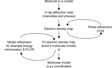
The structures in the atomic and molecular world can be resolved using techniques such as X-ray crystallography, nuclear magnetic resonance (NMR), cryoelectron microscopy, and electron tomography (ET). The data generated by these experiments need to be processed by molecular visualization and modeling software to generate a model of the structure (Lamzin and Perrakis, 2000). Some of the commonly used software in X-ray crystallography includes the CCP4 suite of programs (Collaborative Computational Project, 1994), MAID (Levitt, 2001), ARP/wARP (Cohen et al., 2004), O (Jones et al., 1991), CNS (Brunger et al., 1998), XtalView (McRee, 1999), and X-PLOR (Brunger, 1992). These programs use X-ray diffraction data obtained from a purified protein crystal and generate electron density maps (e.g., CCP4), build the molecular model (e.g., O), and refine the model (e.g., X-PLOR). Many of these programs not only are fully automated, but also allow the user to interact at various points in the analysis. Figure 9.2 shows an outline of the process involved in visualizing X-ray crystallography data. The result of this process is a file containing the 3D orthogonal coordinates (x, y, z) of the refined molecule. These coordinates specify the position of each atom in the molecule within three-dimensional Cartesian space. The coordinates are saved as a file in PDB format, although other formats such as mmCIF are also used (Chapter 10). The 3D coordinates can be used as the input for visualization of the molecule either as a physical or computer-generated model.

3D Coordinates to Molecular Visualization by Physical Models

Despite significant technological improvements in computer graphics, tangible physical models that are not confined to the computer screen are still very useful. Physical models offer an impressionable, persistent, and high impact way to “see” and “feel” the molecule giving the investigator a perspective that promotes understanding and insight that is not always possible with computer graphic models. The building materials used to model molecules include wax, clay, wire, plastic, and wood. Physical models are still very useful in teaching and learning because they provide a multisensory learning experience that also enhances collaboration (Gillet et al., 2005).

Some of the early physical models include Pauling’s space-filled wood molecular models (Corey and Pauling, 1953), Watson and Crick’s wire model of the DNA double helix (Watson and Crick, 1953), and Kendrew’s plasticine “sausage” model of myoglobin (Kendrew, 1961). Eric Martz and Eric Francoeur give a brief, but excellent, history of molecular visualization with pictures of early physical, and computer graphic, molecular models on their history of molecular visualization Web site (Table 9.1).

Recent physical models have been developed by Timothy Herman at the Centre for BioMolecular Modeling, Arthur Olson’s group at the Scripps Molecular Graphics Laboratory, and Richard Garratt at the Instituto de Fisica Sao Carlos (see Table 9.1 for Web sites). The Centre for BioMolecular Modeling uses rapid prototyping techniques such as stereo-lithography, laminated object manufacturing, selective laser sintering, fused deposition modeling, and Z-corp 3D printing to rapidly build high-fidelity molecular models. The Olson group is also investigating the concept of “augmented reality,” which is an interesting approach that combines physical models, computer graphics, and virtual reality techniques (Sankaranarayanan et al., 2003; Gillet et al., 2005). Garratt and Pereira (2006) developed an innovative kit to build plastic cartoon models of proteins suitable for teaching.

The problems associated with most physical models, however, are that they take a relatively long time to build; are not always easy to store, edit, manipulate, or change; have limited interactivity; and quantitative information (such as bond distances and angles) is not readily available. These issues are particularly evident when trying to model large molecules such as proteins. For example, molecule kits are still available to build your own insulin protein (the antidiabetic hormone), but the construction time for this relatively small protein containing 51 residues is in the order of weeks. In contrast, visualizing insulin using 3D interactive computer graphics takes seconds. Computer-generated 3D molecular models readily address the disadvantages of tangible physical models.

3D Coordinates to Molecular Visualization by Computer-Generated Models

Molecular visualization uses interactive computer graphics to generate a virtual 3D image of a molecule on a 2D computer screen from the 3D coordinates of the molecule’s structure. Computer graphics play a central role in producing the image, and the user interacts with the image shown on the computer display. Interactive computer graphics is a large, growing, and actively researched area. It is multidisciplinary and encompasses subjects such as mathematics (particularly geometry and trigonometry), optics (including illumination), psychology (particularly human perception), physics, engineering, computer hardware and software, algorithms, solid modeling, rendering, and animation (Foley et al., 1990). Consequently, we will only briefly discuss the basic aspects of computer hardware, software, and computer graphics techniques to help us understand the process involved in generating the molecule we see on the computer screen.

Computer Hardware

Computer hardware can be constituted of one, or more, of the following components: central processing unit (CPU); CPU-associated memory such as random access memory (RAM) and read-only memory (ROM); storage memory devices (e.g., hard drive, tape drive, and thumb drive); input devices (e.g., keyboard, mouse, tablet, pen), output devices (e.g., printer, plotter, display screen); and communications devices (e.g., modem and network interface).

Three-dimensional computer graphics is complex and involves many calculations and computer operations. Intuitively, we know that it takes more steps to draw a triangular prism (a simple 3D image with four points and six lines) than to draw a triangle (a simple 2D image with three points and lines). If we want to make the prism look “solid,” then we need to provide additional information to specify the surfaces (i.e., the geometrical planes of the prism) and which surfaces are visible from a particular view of the prism. If we also want to add colors, textures, lighting, and other such effects to make the pyramid look more “realistic,” then the number of steps and computer operations increases. Extending the reasoning of this simple example to a protein containing thousands of atoms, it is easy to see how considerable computational power is needed to view the final 3D image. The more information we include in the 3D image the greater the computer power we need to process, visualize, and interact with the image within a reasonable time.

A computer’s “power” is related to the increased speed with which the CPU (variously called achip, microchip, microprocessor, orprocessor) canperformbasic computer operations and calculations. This processing power also depends upon the corresponding advances in other components of the computer, such as higher capacity memory (RAM, ROM, and disk memory), increased speed of internal electronic pathways (data buses), computer architecture, computer input and output devices, and software. In particular, parallel processing architectures (where multiple CPUs and memories are used to increase the number of computer operations that can be performed simultaneously) and dedicated graphics processors have enabled computer graphics to produce stunning photorealistic images (Kerlow, 2004). The relevance of this increased computer power to computer graphics, and to molecular visualization in particular, is that we can generate images with increased clarity, greater interaction, and in less time (so we can get our work done faster!).

The computer display is obviously important, because it enables us to see the computer-generated molecules. During the 1960s, molecular visualization computer systems used vector graphics displays (Francoeur, 2002). Vector graphics is a term used variously to describe the hardware for drawing a 2D shape, a particular image data format, and the mathematics used to represent graphics in software or dedicated graphics processors. The original type of display used with a computer was a cathode ray tube (CRT). A CRT uses an electron beam to irradiate and excite a phosphor to glow on the screen. The line has to be repeatedly drawn or refreshed (at about 30 times per second) to achieve persistent vision, because the phosphor rapidly decays (Foley et al., 1990). The data for this refresh are stored in memory and constituted of the coordinate data and other commands. This is also called a random scan, because the electron beam can scan the complete X-Y dimensions of the available screen, and a point-to-point drawing can occur at any position directed by the order of commands in the vector graphics software. Vector displays are fast and do not use much memory, but can only trace relatively simple lines, planes, and a few colors.

Most current computer molecular visualization systems use raster graphic displays rather than vector displays. Raster graphics is a term used to describe the hardware for drawing a 2D shape, a particular image data format, and particular computer graphic techniques. The image to be displayed on the screen is initially stored in memory (called a frame or refresh buffer) as a two-dimensional array (the raster) of picture elements (pixels) called abitmap. A pixel is a defined area on the display that can be activated and attenuated by the electronic signal generated from the computer (e.g., an electron beam of a CRT). Each pixel can also be activated to show any of thousands or millions of colors depending upon the number of bits (bit depth) used for color in each pixel. A bit depth of 8 bits per pixel would allow 256 colors, while a 24 bits per pixel would allow millions of colors to be displayed. A raster display traces out one horizontal row of pixels at a time (called a scan line) to eventually map the stored bitmap to the screen. The screen has to be repeatedly drawn or refreshed (about 60 times per second) to maintain persistent vision. A computer screen with a resolution of 1280 x 1024 has 1280 pixels per horizontal row and 1024 pixels per vertical row and is considered high resolution. Raster graphics displays use a CRT although newer technologies such as plasma and liquid crystal display (LCD) are also used. Raster displays can be used to show color, complex shapes, volumes, textures, surfaces, and photorealistic images. RasMol is one of the most commonly used molecular visualization programs for raster graphics displays and its name is purported to be a mnemonic for Raster Molecules (see Martz and Francoeur, Table 9.1).

A graphics processing unit (GPU) is a microprocessor dedicated to manipulating and displaying computer graphics. The GPU takes over from the CPU in handling various 2D and 3D graphics tasks. The GPU is responsible for implementing most of the visualization, or graphics, pipeline (see below). Consequently, they help increase the speed of graphics processing and hence molecular visualization. Modern GPUs are also programmable, which means there is more flexibility in manipulating, and presenting, the image. Some molecular visualization applications take advantage of the GPU (e.g., Chimera and VMD), some still depend on the CPU for processing power (e.g., RasMol), and some bypass the GPU altogether to maintain their “platform independence” (e.g., Jmol).

Computer Software

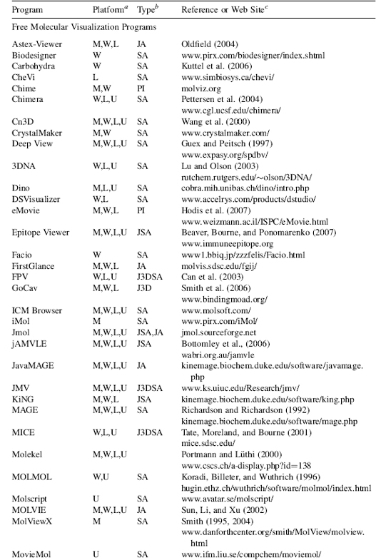
Computer software consists minimally of application programs (also commonly known as “programs” or “software”), such as a molecular visualization program, and an operating system. We will discuss molecular visualization programs in a little more detail later. The operating system provides the basic operating environment of the computer and manages (among other things) the memory (RAM and disk), internal communication with specialized coprocessors such as graphic processing units (GPU), memory storage, and input/output devices. Table 9.2 shows that molecular visualization is carried out on various operating systems and the choice of a particular operating system may depend upon personal preference, reliability, stability, support for extended architectures or modularization, support from developers, graphics libraries or other graphics resources within the system, a suitable user interface such as a graphical user interface (GUI), or commercial considerations. The application software is developed to perform a particular task or range of tasks and works in conjunction with the operating system, the hardware resources of the computer system (e.g., GPU), and other software (e.g., OpenGL).

The Visualization Pipeline

Computer visualization is a complex process that is dealt with by breaking it up into several conceptual stages called a visualization pipeline. The aim of the visualization pipeline is to transform the 3D coordinates of an object (which is a molecule in a molecular visualization program) into a virtual 3D image on a 2D computer display. It is called a pipeline to reflect the fact that it involves an interconnected series of processes where the result of one process usually feeds into the subsequent process. The processes deal with both the shape and the appearance of the molecule. The shape of a molecule is dealt with by the 3D geometric processes of the pipeline and its appearance is dealt with by the rendering processes of the pipeline. Figure 9.3 shows that the pipeline has three general stages: modeling, geometry, and rendering. There are also processes within each stage. The actual sequence of the stages and the type or number of processes within each stage may vary between the application software, the GPU, and the application programming interface (API). An API, such as OpenGL (Angel, 2002), is an interface between hardware and application software. It is a set of rules, and graphics commands, that standardizes the use of hardware GPUs by application software. An API is essentially written into application software and also a GPU. In this way, programmers can write their software to an API, and it should run on any GPU using the same API.

The perception of depth, and hence 3D, of objects presented on a 2D display can be enhanced by many techniques including lighting, motion, color, perspective shading, textures, and shadows. Each of these techniques is applied at particular stages of the visualization pipeline. The modeling and geometry stages of the pipeline deal with the processes that create and define the 3D geometry of an object and are performed by the application program and the GPU. The application defines the particular model, or molecular representation (see the section “Molecular Models”), while the geometry stage involves transformations through various coordinate systems. A computer graphics system capable of producing 3D images generally uses five different coordinate systems: a global, or world, coordinate system; a local coordinate system; a view (eye) coordinate system; a picture (projection) plane coordinate system; and the display screen coordinate system (Mortenson, 1989). We will not go into the details of these coordinate systems here except to say that the initial 3D coordinates of the molecule are progressively transformed into a 2D coordinate system suitable for the computer display and for effective interaction by the user. Other processes (usually applied to a particular coordinate system) determine colors, lighting effects, how the object is clipped to fit on screen (especially if zooming the molecule), and the perspective of the object in geometry stage. Perspective is a particularly useful depth cue and helps create the illusion of 3D from a 2D image. Depth is also dealt with by z-buffering at the next stage of the pipeline (discussed later).

TABLE 9.2. Examples of Recent Molecular Visualization Programs

^aM, Macintosh; W, Windows; L, Linux; U, Unix. No distinction is made between versions, or distributions, of the operating system. Versions may also be run cross platform with suitable simulators, forexample, Parallels Windows simulator for Macintosh.

^bSA, “stand-alone”; PI, “plug in” for a web browser or another program; JA, java applet; J3D, java3D; VR, virtual reality environment; WS, web server.

^cAWeb site URL, reference, or bothis given wherever possible. The “http://” part ofthe URL is omitted for clarity but is implied. Please note that Web site URLs were checked, and operating, before publication, but unfortunately they do tend to change or expire over time.

The rendering and rastorization stage of the visualization pipeline comprise processes that determine the final 3D appearance of the molecule. The aim is to make a realistic image from a geometric model. Many of the effects applied at the rendering stage produce photorealistic images. This is an unfortunate term when applied to viewing molecules since what we are viewing is far from realistic and certainly not photographic. The molecule itself is a model derived from physical data, theory, and prefiltering from X-ray crystallography or NMR spectroscopy. Furthermore, atoms can be depicted as physical objects, and rendering processes can make them look like particular materials (e.g., plastic or metal) with textures, shadows, and colors. These physical attributes obviously do not exist in the real atom. It is all an abstraction and an illusion. However, it is an abstraction that is useful as it can translate into descriptions or predictions of structural and functional properties in the real molecule.

Although screen space is an x-y (i.e., 2D) mapping of a 3D object to the screen, the z-values have been carried through all of the operations in the pipeline. There are various ways to use the depth information implicit in the z-values. One of the more common ways is to store the values in memory called a z-buffer. An algorithm then uses the z-values in the buffer to determine the visibility of parts of the object from a particular coordinate view. A near part of the object might obscure, to some extent, a far section of the object, and the z-buffer algorithm would remove the hidden part of the object from view. Consequently, this helps create the illusion of depth (3D) on the 2D screen.

The final stage of the visualization pipeline takes the rendered image and converts it to a bitmap (a raster graphic) for presentation on a raster graphics display. The bitmap is first stored in a frame buffer (a memory of the bitmap) and then transmitted to the display. Vector graphics can be used in drawing and the geometry of an object, but must ultimately be converted to a bitmap for raster display. Any interaction with the image sends new instructions flowing through the visualization pipeline to produce the modified image. This continual “image-interact-image” loop is an active feedback process that helps the user to interpret, and understand, molecular structure, properties, and function.

Graphics Objects

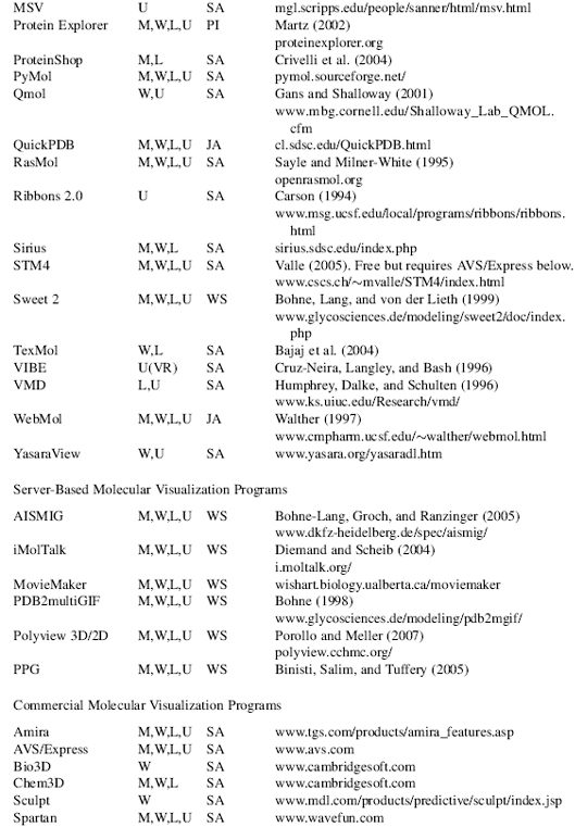
Creating the 2D, and 3D, geometry of a molecule (or other object) involves vector graphics. Vector graphics uses mathematically derived 2D and 3D geometrical shapes called primitives. This is in contrast to raster graphics, which is the representation of images as a collection of pixels and is the type of graphic seen on the computer screen. Vector graphics are eventually converted, by the visualization pipeline, to raster graphics for display on the computer screen. The basic geometrical shapes are described as primitives, because they can be used to construct more complex shapes. The type and number of primitives available in any computer graphics system will depend upon the application software and the GPU. The basic 2D primitives include points, lines, circle, curves, and polygons. The basic 3D primitives are regular polyhedra that include sphere, cylinder, tetrahedron, and cube. All 3D geometric shapes can be created either as polygonal structures or as curved surfaces. A polygon consists of vertices and edges that connect the vertices. Figure 9.4 shows that polygons can be combined in a “mesh” to approximate any shape. A mesh is constructed such that two polygons share an edge. The combination of triangles, in particular, is very useful strategy for forming meshes and building shapes. The greater the number of polygons used to describe a shape, the smoother the shape and the greater the computational power needed.

Curves can also be combined to form a mesh, or curved surface, to model 3D shapes. There are different ways to mathematically determine, and draw, curves with the three most common being: Hermite curves, Bezier curves, and various splines (Foley et al., 1990). Curved surfaces avoid the artefacts that can occur when approximating a shape with polygons. Curves are useful for generating smooth shapes and have been used in the ribbon model for representing protein secondary structures (see section “Molecular Models” below). The general process of combining polygons, or curved surfaces, to create a 3D object is called tessellation. All molecular visualization applications will have these geometric and rendering capabilities, but will vary in how many of these features they offer.

MOLECULAR MODELS

Visualization of molecules using models began as early as 1808 with the introduction of Dalton’s chemical symbols (Figure 9.1) and has progressed to models generated with modern computer graphics. Brief but excellent histories on the development of molecular visualization, and molecular models, can be found elsewhere in articles (Francoeur, 1997; Del Re, 2000; Olson, 2001; Francoeur, 2002; Tate, 2003; Goodsell, 2005), or at Web sites (Table 9.1).

Molecules canbe modeled orrepresented in various ways (Leach, 2001; Goodsell, 2005), and we will discuss some common molecular models in the next section. The models are approximations to reality and are designed to help clarify particular aspects of a molecule’s structure, function, or properties (Laskowski, Watson, Thornton, 2003). Each model gives a different perspective and insight into molecular structure. They also serve as a metaphor for the atomic world we cannot see (Goodsell, 2005) and allow us to compare size and structure of molecules. Structural models of proteins are used to represent the primary, secondary, supersecondary, tertiary, or quaternary structural hierarchy of a protein molecule (Chapter 2, Branden and Tooze, 1999; Banaszak, 2000; Lesk, 2001). They are also used to represent functional domains, binding interactions, solvent-accessible areas, solvent-excluded areas, and as a framework for other physical and chemical properties (e.g., electrostatics). No single model can represent everything. Consequently, the choice of model depends on the particular structure, property, or function that needs to be illustrated.

Most molecular models are represented as physical objects because we can render physical objects in various ways that help clarify, and simplify, structure or properties. However, implicit in this representation are the physics of atomic and molecular structure. While some molecular models are based on quantum mechanics, most structural models are based upon molecular mechanics assumptions (Leach, 2001). That is, the atom is modeled as a hard sphere with the radius of the sphere equal to, or some multiple of, the atom’s van der Waals radius. Some molecular models such as the ribbon, backbone, and trace models may not represent atoms as spheres, but molecular mechanics assumptions are usually inherent in the model or in the data used by the model. Covalent bonds are represented (as they are in the usual 2D chemical graphs) as line segments, or 3D cylinders, joining each of the atoms. We will discuss aspects of the more common molecular models later.

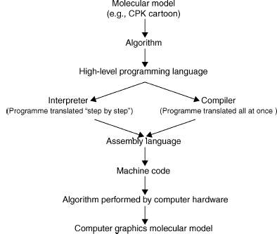
Figure 9.5 shows that a molecular representation starts out as a fundamental mathematical, chemical, or physical chemistry model that is converted into an algorithm and written in a particular programming language. This algorithm is then either interpreted or compiled into machine code read by the computer. The efficiency of the application software, and the representation of a particular molecular model, is intimately related to the efficiency of the algorithms used in the software (Harel, 1998).

An algorithm is a precisely defined procedure for accomplishing a particular task. An algorithm can be likened to a recipe for baking a cake. However, in computer graphics the recipe is coded in a programming language, rather than a written document, and is implemented by a particular application program (e.g., molecular visualization program) on a computer system. The programming language can change, but the algorithm always remains the same. The efficiency of an algorithm is measured both by the time and the amount of storage space (memory) needed to perform a particular process (e.g., draw a CPK atom). Memory space is determined by the amount of data and the number of storage locations needed by the algorithm to perform the particular process. Time is determined by the number of elementary steps needed by the algorithm and the speed with which the CPU can perform those steps. The“big-O” notation(for “order of” ) describes thedependenceof an algorithm on both time and space. For example, an algorithm that is described as O(N) performs N elementary instructions, and its running time, or memory requirement, is linear with N. The “big-O” notation can give some idea of the speed and the efficiency of the algorithm, but the actual run time will also vary with the computer architecture and on the size of input data (Harel, 1998). The importance of this to molecular visualization is that some molecular models run faster, or slower, than others depending upon the complexity of their algorithms and their implementation on the graphics hardware. We will now discuss some of the common molecular model algorithms used in molecular visualization.

Wireframe, Stick, CPK, and Ball and Stick

Figure 9.6 shows some of the common molecular models used to represent protein structure. The wireframe model is the simplest molecular model where line segments represent bonds and the atoms are at the vertices of the line segments. It is often used as the default model when a molecule is first opened by, or loaded into, a molecular visualization application. It is faster to render because it needs only the coordinates of the atoms to draw a line segment (one of the graphics primitives) between them. Consequently, it takes much less time and memory to process than a more complex model and leaves the CPU more time to respond to other user commands. The disadvantage of a wireframe model is that it is difficult to discern color and 3D structure especially when viewing larger molecules such as proteins.

The stick model (derived from physical models developed by Dreiding, 1959) can be seen as essentially a thicker wireframe where the bond is represented as a cylinder. This is also called a “licorice” model in some molecular visualization applications (e.g., VMD). The cylinder can be drawn by increasing the diameter of the line segment or by rendering a cylinder using the geometric primitives available with the application or the GPU. Color and other effects can be added to the model. The issues with this model are the same as for the wireframe molecular model.

The CPK model takes its name after its originators and is also known as the space-fill model (it is also a color scheme, see below). It was derived from wood and plastic physical models developed by Corey and Pauling (1953) and later Koltun (1965). Each atom is represented as an opaque sphere with a radius equal to its van der Waals radius. The spheres can be rendered as a 3D primitive, as tessellated polygons or curved surfaces, depending upon the molecular visualization program and the GPU. Color, lighting, transparency, textures, shading, and other effects can also be added to the spheres. Consequently, greater computation is needed to render the model especially in proteins where there are thousands of atoms. Algorithms have been developed to increase the speed of rendering CPK models (Schafmeister, 1990). If the molecule is moved, then the CPK model may be rendered with open meshes (small number of polygons), dots, or the CPK model is removed altogether. Thus, processing time is not unnecessarily consumed by the need to continuously render and redraw the screen with each movement of the molecule. The CPK model implies volume and is also one of the first surface representations of a molecule. It is useful for showing the size and shape of a molecule, for showing when atoms may collide in certain conformations due to steric hindrance, and for showing cavities. However, it can also obscure details and cause visual clutter when used to model larger molecules and proteins (Francoeur, 1997).

The ball and stick model is a hybrid between a stick model and a CPK model. Bonds are represented as cylinders and atoms as spheres or sometimes ellipsoids (Burnett and Johnson, 1996). Unfortunately, perhaps, some molecular visualization applications have also called this a CPK model (e.g., VMD). Color, lighting, textures, shading, and other effects can be added to the both bond cylinders and atom spheres. However, the radii of the atom spheres are usually much less than the true van der Waals radii to reduce visual clutter and enable faster rendering. The ball and stick model is useful for information on topology and for measuring bond angles, torsional angles, and bonds lengths. However, Figure 9.6 shows that the ball and stick model still creates visual clutter when used to model proteins.

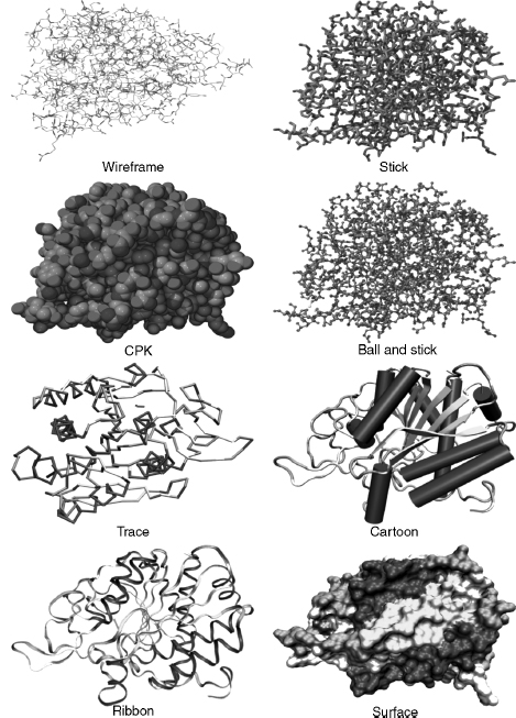
Wireframe, stick, CPK, and ball and stick molecular models may be considered “all-atom” models in that each atom in the protein is explicitly included in the model. The following molecular models involve algorithms that use a particular subset of atoms. They were designed to simplify and clarify protein structures and show elements of structure obscured by all-atom representations.

Backbone, Trace, Cartoons, and Ribbons

The backbone model (possibly based on physical models of Rubin and Richardson (1972) and Keefe and Howe (1973)) was introduced for proteins and is conceptually similar to the stick model for smaller molecules. The backbone of a polypeptide is minimally constituted of the carbonyl carbon, the alpha carbon, and the amide nitrogen of each residue (Chapter 2). However, the backbone model’s algorithm uses line segments to join each consecutive alpha carbon in the polypeptide. The advantages of this model are that it simplifies the structure; it avoids visual clutter; it is faster to render; it can reveal elements of secondary structure such as helices, strands, and turns; it can show the conformation and folding of the polypeptide chain; it is useful in tracing electron density maps; and can be used to determine protein dynamics (Higo and Umeyama, 1997). A disadvantage is that it is visually less impressive than cartoons or ribbons.

The trace model is similar to the backbone model except that spline curves are used to generate the trace through the alpha carbon atoms. The mathematics of the curve may mean that the curve does not exactly intersect the coordinates of each alpha carbon, but this makes the model look smoother. The backbone and trace models are also useful for protein structure comparison techniques (used in threading and homology modeling), where usually only the coordinates of alpha carbons are considered (Johnson and Lehtonen, 2000).

The cartoon models of proteins were derived from hand drawn models of protein secondary structures by Richardson (1981, 1985a and 1985b). The computer graphics for cartoon models were further developed by Kraulis (1991) in the program Molscript. The advantages of cartoon models are as for the backbone model above. In particular, it simplifies protein structure to reveal the direction of the protein chain, protein folding, and elements of secondary, supersecondary, and domain structure. Secondary structure determination is important in categorizing proteins in both the CATH and SCOP databases (Chapters 17 and 18). The cartoons can be rendered as solid graphic objects (e.g., helices as cylinders and p-strands as broad arrows) and have various lighting, shading, and other effects applied.

Ribbon models were derived from Richardson’s hand drawn models (Richardson, 1981; Richardson, 1985b) and later developed by Carson (Carson and Bugg, 1986; Carson, 1987). They could also be labeled a “cartoon,” butribbons are usually listed as a separate rendering option in molecular visualization programs. The justification is based on the mathematical model, and algorithm, used to graphically create the ribbon that is based on a B-spline curve. The peptide planes of the peptide bond are used as the coordinates for the spline. Initially, the ribbons were generated as separate spline line segments winding their way down the polypeptide chain (Carson and Bugg, 1986) but later the splines were used to form curve patches that could be rendered as solid ribbons (Carson, 1987). Later development of the ribbons algorithm allowed ribbons to take full advantage of raster computer graphics capabilities including color, transparency, shading, and lighting that produce ribbons of varying styles (Carson, 1994).

Surface Models

That part of a protein exposed to the surrounding environment of solvent, and other molecules, is generally described as its solvent-accessible surface. It is this surface and its constituent atoms that are important to the protein’s function (Via et al., 2000). The volume or bulk of a protein is also implicit with some surface models, and this helps to define the shape and size of the molecule as well as the extent of a particular molecular property (see below). One of the first models to show explicit surface boundaries and volume was the CPK model discussed above. However, this is an all-atom model, and it does not clearly discriminate between those atoms that are on the surface available to interact with the surrounding solvent and those that are buried. Algorithms are used to smooth the “bumpy” all-atom representation, reduce the clutter inherent in the CPK model, and produce an overall shape for the protein that represents its surface topography.

Various methods have been developed to describe a protein’s surface (Blinn, 1982; Connolly,; Max, 1984; Goodford, 1985; Richards, 1985; Goodsell, Mian, and Olson, 1989; Goodsell and Olson, 1990; Agishtein, 1992; Laskowski, 1995; Sanner etal., 1996; Cai, Zhan, and Maigret, 1998). Michael Connolly has written an excellent review on the development of surface models on the NetScience Web site (Table 7.1). We will only briefly discuss some of the main concepts and algorithms.

Lee and Richards (1971) described a protein’s solvent-accessible surface by using the “rolling ball” algorithm. The algorithm uses a sphere of a particular radius to roll over the surface atoms of the protein. The radius of the sphere can be altered, but it is usually set to the 1.5 Aradius of a water molecule. Each atom is represented by its van der Waals radius, and the center of the sphere traces out the solvent-accessible surface. Connolly (1983a 1983b) further developed this algorithm to run on computer graphics systems and describe the related concept of the solvent-excluded surface (otherwise known as the molecular surface). The solvent-excluded surface is where the atom’s van der Waals radius comes into contact with the probe and forms the boundary for the excluded volume. An alternative approach (called a “volume-based” approach) to determine the accessible surface of a protein uses a probe to scan the complete 3D internal, and external, space of the protein, rather than just rolling it over the surface (Goodford, 1985; Goodsell and Olson, 1990).

Surfaces are complex graphical objects and can be rendered as dots, meshes, or solids (where the mesh and solid can be constituted of tessellated polygons or curves). Color, lighting, textures (Teschner et al., 1994), shading, and other effects can be added to the surface. Surfaces take longer to render, and research is directed to develop algorithms to reduce the rendering time (Sanner, Olson, and Spehner, 1996; Bajaj et al., 2004).

Properties of a molecule such as electrostatic potential, hydrophobicity, and some noncovalent interactions can be modeled as a surface plane or as a surface that defines a volume in or around the molecule. The surface plane approach maps the property to a curved plane with proximity to the residue or atom comprising that property. The plane can be rendered with different colors or textures. The surface volume approach maps the property to an existing surface (such as a Connolly surface), either as acontiguous “density cloud” (also known as volume rendering), or as 3D isovalue contour (Goodsell and Olson, 1989; Henn et al., 1996; Olson, 2001; Holtje et al., 2003; Goodsell, 2005; see also O’Donnell Web site listed in Table 7.1). Some field-like properties, such as electrostatics, vary in size and direction both in and around the molecule. Consequently, it usually is more informative to display properties as density clouds, or 3D isovalue contours, with varying volumes in and around the molecule. The extra information provided by molecular properties can be visualized by varying the opacity, texture, or color of the rendered volume or surface.

Colors, Covalent and Noncovalent Interactions, and Hydrogen Atoms

The CPK color scheme was based upon the colors of the space-filling models developed by Corey and Pauling (1953). In this scheme, carbon is light gray, nitrogen is light blue, oxygen is red, hydrogen is white, and sulfur is yellow. Many other color schemes can be used to highlight other features, such as atom types, a structural part of the molecule, or molecular properties (e.g., charge and polarity). Most molecular visualization programs enable the user to define colors.

Single covalent bonds are usually represented as line segments or cylinders in models and can either be calculated by the molecular visualization program or generated directly from the “CONECT” records of the PDB file. The molecular visualization program calculates the van der Waals radii of two adjacent atoms and if the distance is less than the sum of the van der Waals radii of the two atoms, then a bond is drawn between them. Double bonds are not usually represented in the PDB file, so the molecular visualization program also has to calculate these using the distances between atoms where the length of a single bond is greater than a double bond that in turn is greater than a triple bond.

Noncovalent (nonbonded) interactions occur within protein structures, between proteins, and between proteins and ligands and include hydrogen bonds, hydrophobic interactions, ionic interactions, aromatic interactions, and metal complexation (Bohm and Schneider, 2003). Hydrogen bonds (Pimentel and McClelan, 1960) are usually modeled, because they are a common interaction and have important roles in protein structure and function (Jeffrey, 1991). The geometry of the hydrogen bond is also well known, and as such, it is relatively easy to design algorithms to detect and display them. Hydrogen bonds are calculated using bond angles, bond distances, and sometimes with reference to atom types. If two atoms are within particular bond distances and bond angles, then a dotted line is usually drawn to signify the bond. Molecular visualization applications may have different ways of determining and drawing the hydrogen bond. The hydrogen atom locations (see below) may also have to be calculated before hydrogen bond placement.

Hydrophobic interactions are also important in protein-protein interactions (Mueller and Feigon, 2002), protein folding, and protein stability (Hendsch and Tidor, 1994; Wimley et al., 1996). Various criteria can be used to determine the hydrophobic and aromatic (Kolomeisky and Widom, 1999; Sacile and Ruggiero, 2002) propensities of proteins, and these can be mapped as an isovalue surface or mapped on to an existing surface (see Surfaces above).

Aromatic interactions, such as pi-pi (McGaughey, Gagne, and Rappe, 1998) and pi-cation (Ma and Dougherty, 1997), have important roles in enzyme-substrate interactions, ion channels, and membrane receptors (Kumpf and Dougherty, 1993; Dougherty, 1996; Ma and Dougherty, 1997; Gallivan and Dougherty, 1999; Pletneva et al., 2001). However, the geometry and conditions for these interactions is not always straightforward, and it is difficult to design appropriate algorithms to detect them in protein structures. Consequently, they may not always be available as models in molecular visualization applications.

Many protein structures solved by X-ray crystallography do not have implicit hydrogens because the resolution of the technique does not allow for definitive identification of the small hydrogen atom’s location. Consequently, the molecular visualization program has to calculate the position of the hydrogen atom in the structure. The calculation is usually based on the atom type. The atom type is a classification of atoms based upon their chemical environments and bonding propensities. For example, carbon can be classified as sp³hybridized, sp² hybridized, sp hybridized, aromatic, or carboxylate carbon. Each atom type will have a defined geometry and will bond to a different number of hydrogen atoms.

Animations

Animation can be a useful and powerful molecular visualization tool (Max, 1990; McClean et al., 2005; Breithaupt, 2006; Hodis et al., 2007). The addition of movement adds another dimension to help clarify and communicate information about molecular structure and function. Molecular animations are not purely artistic representations but are based upon actual 3D coordinates and molecular dynamics. The Database of Macromolecular Movements (Echols, Milburn, and Gerstein, 2003), which is a collection of data on the flexibility of protein and RNA structures, is an example of the utility of animation. RasMol, one of the earliest molecular visualization programs, can produce simple animations using scripts or animated gifs (Bohne, 1998). MovieMol (Table 7.2), MovieMaker (Maiti, Van Domselaar, and Wishart, 2005) and eMovie (Hodis et al., 2007) are some of the programs specifically designed to produce molecular animations. Alternatively, generic animation programs such as, Macromedia’s Flash, Apple’s QuickTime, or Autodesk’s Maya, can be used to produce animations based on actual 3D coordinate data. We will not go into the details of making animations, but Table 9.1 lists a few of the many Web sites that feature animations for both research and education.

MOLECULAR VISUALIZATION PROGRAMS

Molecular visualization programs enable molecules to be viewed as different models or molecular representations that reflect underlying physical, chemical, or structural principles. The user can also manipulate, and interact with, the molecular image to control both its content and appearance. Molecular visualization applications vary considerably in the number, and range, of features available for interacting with, and viewing, the molecule. However, most programs have the ability to import, export, and save molecules in PDB and other molecular file formats; display the molecule in standard molecular model types (see above); move the molecule by rotation and translation; scale (zoom in or zoom out); selector “pick” parts of the molecule; and color the molecule according to various standard or nonstandard color schemes. Additional features may include other types of molecular model types, molecular surfaces, rendering effects (such as lighting, shading, depth cues, and perspective), stereo view, structural alignment, and molecular modeling tools (e.g., the ability to mutate residues and build molecules). Most programs process the input files by using internal algorithms to analyze the structure and check such things as atom distances, bonds, and connectivity. Any problems would either be automatically fixed or reported to the user.

Most molecular visualization applications have a graphical user interface and the user can directly interact with the program through pull-down, pop-up, or contextual menus, and mouse actions. Other applications (e.g., Molscript) will have a command line interface that accepts specific commands, or a command language, to control the function of the program and the molecule display. Command line interfaces allow the user some flexibility in manipulating and displaying the molecule that would otherwise not be available as a menu item. Some applications will be able to accept a series of commands (called scripts or macros) stored in a text file that can be loaded by the program to automatically execute the commands. These command line interfaces, with scripting, allow the user to automatically perform complex or repetitive operations. Finally, some applications have the best of all worlds and have a combined GUI and command line interface (e.g., RasMol, jAMVLE).

Most molecular visualization programs will display a range of small molecules, proteins, DNA, and RNA. However, there are also programs (see Table 9.2) that specialize in visualizing particular structures such as 3D immune epitopes (Epitope Viewer), large macromolecular assemblies (Chimera or TexMol), DNA (3DNA), and carbohydrates (Carbohydra or Sweet II).

Molecular Visualization versus Molecular Modeling

What is the difference between a molecular visualization program and a molecular modeling program? A molecular modeling program has the ability to construct, simulate, and predict molecular structures, properties, or functions. They can measure and manipulate the geometry of the molecule’s structure, calculate various molecular properties according to particular force fields, test various molecular conformations by performing energy minimizations, and compare structures (e.g., protein-protein, protein-ligand, or protein-drug). We have already seen that various molecular models are used by molecular visualization applications. Some molecular visualization programs also have the ability to construct molecules and perform energy minimizations. Thus, we could say that some molecular visualization programs also support molecular modeling. However, the emphasis of a molecular visualization program is the visual representation of molecular structure and properties. This could also be envisaged as the graphical “front end” of a molecular modeling program where the “back end” is the underlying computational ability of the molecular modeling program.

Types of Molecular Visualization Programs

Table 9.2 shows that there are many software programs available for 3D molecular visualization that operate on a variety of computer platforms. These are used as standalone programs (e.g., Deep View, Mage, RasMol, and VMD), integrated within a web browser (e.g., Chime and Protein Explorer), as java applets integrated within the web browser (e.g., Jmol, WebMol, and QuickPDB), as stand-alone Java-based programs (e.g., Jmol, jAMVLE, KiNG, and Cn3D), as interactive server-based programs (e.g., AISMIG and iMolTalk), as an integral component in a suite of other bioinformatics (e.g., Vector NTI, CICbio, and Geneious) and molecular modeling (e.g., Catalyst and Sybil) programs, or as a distributed system (Zhu et al., 2004).

Molecular visualization programs can export molecule files in various formats that can then be used by other programs or online servers. For example, more fully featured rendering programs, such as Pov-Ray (Table 9.1) and Render3D (Merritt, 1994), are often used to produce publication quality molecular images from molecular files. Molecules can also be visualized by online generation of pictures or animations (Binisit et al., 2005), by generic programs such as QuickTime, or by viewers for web-based markup languages such as virtual reality modeling (or markup) language (VRML) and X3D (Liu and Sourin, 2006; Willis, 2006). Molecular visualization programs can be implemented in virtual reality environments (Luo et al., 2004; Ferreira, Sharma, and Mavroidis, 2005; Gillet et al., 2005), collaborative virtual environments (Bourne et al., 1998; Tate, Moreland, and Bourne, 2001; Marchese, Mercado, and Pan, 2003; Chastine et al., 2005), and with haptic technology (Sankaranarayanan et al., 2003; Wollacott and Merz, 2007). In addition, software development toolkits such as the MBT toolkit (Moreland et al., 2005), and component-based software (Sanner, 2005), offer a flexible and modular approach to quickly develop molecular visualization software. These can be used to cater for new visualization methods, new data types (such as large macromolecular assemblies), and to offer the software through the Internet.

There are advantages and disadvantages for each type of molecular visualization program. The stand-alone applications take full advantage of the computer system’s hardware and software configuration, and this leads to more options available for visualization. This includes a greater range of molecular models, various interactive tools for editing and modifying molecules, and powerful rendering capabilities. However, the stand-alone applications may not be available for all computer platforms (i.e., limited “portability”); need continuous development to keep up with changes in operating software, computer hardware, data types, and molecular visualization concepts; can be awkward to use in conjunction with web-based educational materials (Bottomley et al., 2006); have limited ability to be customized; and are usually offered “as is” to the user.

Web browser integration programs (e.g., Chime), and some Java applets, offer good integration with web-based educational materials. However, they can have compatibility issues with different web browsers or computer platforms. They also do not take advantage of the operating system software or hardware and, consequently, may offer relatively limited options for visualization or interactivity.

Java applications offer independence from either the web browser or the operating system. Java is an interpreted language, and its programs are compiled into a “virtual computer” called the Java Virtual Machine. The Java Virtual Machine, and Java interpreter, needs to be installed on the computer platform to run Java code. Java’s independence from the operating system means that software can be developed once and used with minimal problems on most computer platforms (i.e., Java offers “portability”). It also provides some protection from system crashes, because it operates through the Java Virtual Machine that essentially acts as an interface to the operating system. Furthermore, Java applications can be flexible, modularized, and offered as open-source software (e.g., Jmol). This allows them to be updated, and modified, by the scientific community to cater for new developments in molecular visualization. The lead time for implementing new developments in open-source applications depends upon the enthusiasm of the scientists working on the software, but it can be relatively fast compared to updates to stand-alone applications. Jmol, in particular, has a growing and enthusiastic community of developers (e.g., www.jmol.org) that bodes well for its future use in molecular visualization. Jmol does not need a GPU, and this can be an advantage for those computer systems that do not have a 3D graphics card. However, this can also prevent it from taking full advantage of the operating system software and graphics accelerating hardware.

General VRML, or X3D, viewers may have compatibility issues with computer platform or browsers, offer limited interactivity, and may not always use the computer systems GPUs. A recent development is ProteinX3D (Willis, 2006; Willis, 2007), which is a Java program that uses XML data from the PDB database to visualize proteins.

Applications of Molecular Visualization

Molecular visualization is a powerful concept and tool to simplify, clarify, model, analyze, illustrate, and communicate molecular structure, properties, and function. A molecular visualization arises not only as a result of a dedicated interactive display program (e.g., RasMol), but also as a result of computational analyses generated by many other programs (e.g., from molecular modeling or bioinformatics programs). Consequently, molecular visualization can be applied in myriad situations (too many to list here), and some examples are art (Gaber and Goodsell, 2000; Goodsell, 1991; also see Table 9.1 for the Web sites of the Molecular Graphics Art Show, “Artn,” and Biografx), education (Gilbert, 2005; Bottomley et al., 2006), sequence or structure alignment (Chapter 16; Catherinot and Labesse, 2004), protein docking (Chapter 27), structure superposition (Chapter 16; Sumathi et al., 2006), structure-based drug design and development (Meyer, Swanson, and Williams, 2000; Chapter 34), viewing binding cavities (Smith et al., 2006), viewing multiple protein-ligand complexes (O’Brien et al., 2005), viewing protein interfaces (Teyra et al., 2006), mapping motifs to structure (Bennett, Lu and Brutlag, 2003), homology and homology modeling (Chapter 30), protein classification (Chapters 17 and 18), viewing ligand binding modes (Chapter 27; Ivanov, Palyulin, and Zefirov, 2007), structure prediction (Chapters 28, 29, 30, 31, 32), determining drug efflux mechanisms (Kiralj and Ferreira, 2006), and even used as a “toy” (Laszlo, 2000).

Issues with Molecular Visualization

Most molecular visualization applications are robust. This means that they are usually reliable, do the job required of them, and are not prone to crashing your computer. Consequently, users tend to trust the software and the result produced. However, there are philosophical (Hendry, 1999; Francoeur, 2000; Zeidler, 2000) and practical issues with molecular visualization. In particular, there is a danger in accepting any biological software, including molecular visualization applications, at face value. Molecular visualization applications can contain errors and may interpret data in different ways. For example, RasMol often incorrectly lists the number of polypeptide chains in its summary window, because it interprets nonpolypeptide hetero groups as a chain.

There are also issues in the design of the software. The user interface varies considerably between different molecular visualization applications (see above). The interface can sometimes be rudimentary (e.g., a command line), complex (e.g., contain various options and parameters), and may contain language (e.g., computer graphics terminology) not immediately understandable by the biologist. This can cause confusion especially if the user lacks the relevant knowledge. Consequently, users may only choose the “default” parameters supplied by the software. They may not know how to adjust parameters to refine their analysis, nor the effect that such changes may have on their results (Bottomley, 2004; Goodsell, 2006). This could lead to inappropriate application of the software and questionable relevance and validity of the results. Default parameters also differ between molecular visualization programs, and choosing the default space-filling representation in one program (e.g., jAMVLE) can result in a completely different representation in another program (e.g., CrystalMaker).

As Goodsell (2006) has correctly pointed out, there is the danger of confusing the “image” with science. Optical illusions demonstrate that our visual acuity is so persistent that we sometimes “see” things in images that are not really there. This can be an asset when we want to create the illusion of volume in an atom on a computer screen, but it can be a liability when trying to make valid interpretations of images generated from scientific data. Moreover, molecular visualization software is built from assumptions inherent in its algorithms, mathematics, engineering, and programming. Consequently, software is not always as objective as we may like to believe and the results are necessarily an approximation to reality. Visualization is both objective and subjective. It is objective in that it uses raw data, but it is subjective depending upon how we transform, and interpret, the raw data. There will always be a compromise between the two. That is, we can try to be as objective as possible in generating our data, but as soon as we start transforming the data, we necessarily presuppose some model or theory. Our interpretation of that transformation will be subjective based on the underlying model or theory. The user can also choose a particular molecular model, or rendering technique, based only on personal preference. This will bias the image in some way and may be chosen to satisfy a particular audience (Goodsell, 2006). For example, an austere, precisely defined, molecular representation would be appropriate for a knowledgeable scientific audience, but a more colorful, and artistic, representation would be appropriate for a nontechnical audience. Thus, it is possible to use molecular visualization to inadvertently, or even deliberately, mislead the intended audience.

There is also a temptation to assume that we do not have to know how the software works as long as it gives the results we are seeking. However, we should carefully consider many factors that may affect the efficacy, the robustness, and the biological relevance of the software as failure to do so may result in misuse (Bottomley, 2004). The image on the computer display is the final stage of the molecular graphics visualization pipeline, but it is the penultimate stage in interpretation. Visual images are powerful, but it still needs an experienced, knowledgeable, biologist to interpret the result and give it biological relevance and validity.